DNA by Design: De novo Computational Framework for DNA Sequence Design and Nanotechnology

Simon Vecchioni^{1, 2}, Ruojie Sha², Nadrian C. Seeman^{2, †} Lynn J. Rothschild³ and Shalom J. Wind^4,*

¹Columbia University, Department of Biomedical Engineering, New York, United States
²New York University, Department of Chemistry, New York, United States
³NASA Ames Research Center, Planetary Sciences Branch, California, United States
⁴Columbia University, Department of Applied Physics and Applied Mathematics, New York, United States
E-mail: sw2128@columbia.edu
*Corresponding Author
^†Professor Seeman passed away during the preparation of this manuscript.

Received 23 February 2022; Accepted 11 October 2022; Publication 03 January 2023

Abstract

Chemical analysis of metalized DNA has made it quite clear that traditional models of DNA thermodynamics are insufficient to predict and control self-assembly in the context of orthogonally-paired nucleotides. Recently, there has been an increase in reports of Watson-Crick assembly of DNA wires and nanostructures [1–4]. The ability to add or remove pairing rules between nucleobases toward non-Watson-Crick, or orthogonal, self-assembly alters the fundamental language of DNA assembly: this change in behavior necessitates an accompanying shift in computational design. We begin by exploring the state-of-the-art in DNA modeling, and include both sequence analysis and sequence design practices. We then start from first principles and establish a mathematical basis for heterostructure and ‘nmer’ analysis in connected DNA networks that operates without assumptions about nucleobase parity. A generalized search algorithm is then constructed in Matlab and implemented using evolutionary techniques. We then discuss DNA nanostructure design criteria, operation efficiency in differentially-connected networks, and the application of computationally-aided sequence design for nanotechnological applications. We design a double crossover DNA motif with a silver base pair modification as a test case, and demonstrate successful model implementation. In sum, we present a novel computational framework for geometry-informed optimization of DNA networks. This tool is meant to enable design of both linear and nonlinear polynucleotide assemblies with inherent modularity for base parity, metalation, or more exotic nucleotide substitutions that may arise from advances in synthetic biology, nanomaterials and nanomedicine.

Keywords: .

1 Use of Computational Modeling in DNA Sequence Design

1.1 DNA Hybridization by Design

DNA hybridization is an emergent property that is predicated upon the base complementarity of two or more oligonucleotides [5]. The formation of a double helix or other nucleic acid heterostructure requires the association of typically more than three complementary nucleotides via hydrogen bonding [6–8]. Qualitative analysis shows that in canonical, “Watson-Crick” (WC) pairing environments, deoxyadenosine (dA, or A) will form two hydrogen bonds with deoxythymidine (dT, or T), while deoxyguanosine (dG, or G) will form three hydrogen bonds with deoxycytidine (dC, or C). Formation of consecutive antiparallel (5’-3’: 3’-5’) base pairs will allow the assembly of a B-form double helix with a periodicity of 10.4 base pairs (bp), or 3.57 nm in neutral pH [9]. In an expansion of WC parity, it has been more recently shown that the introduction of the metal ions Ag${+}^{}$ and Hg${2+}^{}$ will mediate the formation of homonucleotide bonds between opposing C and T bases, respectively [10, 11].

Alternative structures can be formed, by either forcing parallel base pairing (5’-3’: 5’-3’) to form a left-handed Z-form helix [12]; by dehydration to form an A-form helix [13]; or through the introduction of homonucleotide repeats, such as protonated polycytosine assumption of an i-motif structure at acidic pH [14], or polyguanosine assumption of a tetraplex helix over long distances in the presence of divalent counterions [15]. More fundamental to the self-assembly of macromolecular nanotechnology, proper design of multi-oligo systems can allow for helical branching, an idea first proposed in 1982 by Nadrian Seeman [16], and which has been expounded upon many times over in subsequent decades [16–18]. Complex structures, called DNA origami, have been subsequently created using large ssDNA viral plasmids and hundreds of short (20 nt) staple oligos to pinch the template into desired conformations, a technology invented by computer scientist Paul Rothemund in 2006 [19, 20].

With only four nucleotides to work with, and only two canonical base pairs, the design and construction of DNA oligomers with topologically-exclusive thermodynamics is a significant challenge. In the same way that single amino acid mutations can inhibit proper protein folding to generate disease states, imprecise DNA sequence design can promote the formation of thermodynamic mush, rather than meticulously prepared lattices or networks.

Each DNA nanotechnology group has their own method for sequence design, driven by a need to promote hybridization over tens of nanometers with ever-increasing geometric complexities to form vast arrays of two- and three-dimensional structures, including rings, coils, crystallographic arrays, and semiconducting cubes [21–26]. For example, the field standard used by the Seeman group is a legacy FORTRAN algorithm, SEQUIN, which allows for the design of structures in the command line with iterative, click-through construction [27]. This algorithm has driven the generation of oligomer sequences for three decades, but does not have the modularity to tackle non-canonical or artificially-expanded genetic coding for modern nanostructure design. The Rothemund group has used variety of computational tools to design non-interfering DNA oligomers for origami structures, first using unpublished Matlab code, and then switching to origami tool caDNAno [28]. UNIQUIMER 3D is a more modern tool that integrates 3D structure with sequence design, allowing for more interactive structure design, but this tool again suffers from constraints around base parity and part parameterization [29]. A field-unifying, modular sequence design tool has yet to emerge that covers the diverse needs of researchers, though there are many examples of software packages that address different stages of the design process [30–33].

Comprehensive oligonucleotide design parameters were driven largely by the expanding needs of molecular biologists and the researchers at the forefront of the Human Genome Project: it was necessary to design DNA and RNA primers to amplify particular fragments of DNA [34]. The design of effective polymerase chain reaction (PCR) primers required the application two critical pieces of information: (1) the oligo dissociation temperature or melting temperature and subsequent matching within $+/-$2${\circ }^{}$C of the melting temperatures for the forward and reverse primers; and (2) the exact size, and subsequent minimization of, unwanted primer heterostructures, or ‘primer dimers’ [30]. Modern software packages for molecular biology include primer design tools that execute iterative optimization to fix these two parameters [30]. The requirement of accurate, sequence-specific melting temperatures produced a strong drive to fully elucidate nucleic acid thermodynamics, while the need to design DNA sequences with ever-increasing genetic databases covering millions of nucleotides spurred the development of machine learning and iterative optimization approaches to multi-objective algorithmic design.

1.2 DNA Thermodynamics

It was realized early on that the thermodynamics of individual nucleotides in long oligo chains are not linearly-independent; rather, there are adjacency effects along the macromolecule unrelated to the contribution of hydrogen bond energy stored in base pairs. The best example of this resulted from analysis of dG:dT mismatches, which are considered a wobble base pair generally recognized and excised by DNA repair enzymes [35]. The confounding effect of G-T mismatches on overall strand formation served as a model for eventual analysis of adjacency, where sets of three consecutive nucleotides were analyzed in a frame, using the 3-nt codon/anti-codon set found in the ribosome as a template.

It was through painstaking thermal denaturation analysis performed via UV-Vis spectrophotometry in the SantaLucia laboratory in the late 1990s that a nearest-neighbor model of DNA assembly was elucidated, using sets of two—not three—adjacent nucleotides summed axially along the oligonucleotide [35, 36]. In this approach, each pair of adjacent bases contributes to the energy profile of the oligomer, such that the energy contribution of each nucleotide will be accounted for twice: once for each neighboring DNA base. The terminal bases, left out of this accounting regime, instead contribute strand initiation and termination energies, namely the energy required to form the first base pair and break the last base pair in a DNA duplex. Extensive analysis showed that each set of nearest neighbors is linearly-independent, providing a unique enthalpic, entropic and energetic contribution. Studies soon followed to add corrections for ribonucleic acid (RNA), locked nucleic acid (LNA) and mixed, non-specific bases [37, 38]. In this way, the free energy of any duplex or primer dimer could be calculated to a high degree of accuracy.

Unfortunately, a reasonable extension of the relatively simple free energy calculation to duplex melting temperature was not achievable. Simplistic formulas for melting temperature prediction were utilized, one of the most popular using the energetics and the concentration [39]: the nearest-neighbor sequence enthalpy ($\mathrm{\Delta }$H), the nearest-neighbor entropy ($\mathrm{\Delta }$S), R${g\mathit{}a\mathit{}s}_{}$ (1.987 cal/Kmol), and the concentration of the oligomer in moles/L ([oligo]). The final temperature in degrees Kelvin is independent of any contributions of salt stabilization and pH, and it is therefore only useful as a reference number in very rough calculations. Other forms of this approach are also feasible, using the GC concentration, the Na${+}^{}$ concentration, and other factors, but it was the DNA sequence design companies, in an effort to provide reliable, competitive products, who funded and carried out the experiments necessary to identify a comprehensive formula for buffer-specific melting temperature in arbitrary oligonucleotides.

Working with oligonucleotide synthesis company IDT-DNA to predict primer melting behavior for customers, Owczarzy and colleagues provided the most complete melting analysis of nucleic acids to date [40]. This model corrects for buffer counterions at intermediate concentrations by separating samples into three regimes based on the ratio of monovalent to divalent cation buffer species (constant R, in their literature). Different constants of varying complexity are applied in Na${+}^{}$-heavy, Mg${2+}^{}$-heavy, and balanced situations, relying on the oligo concentration, salt concentration, pH, and GC content (sample data shown in Figure 1).

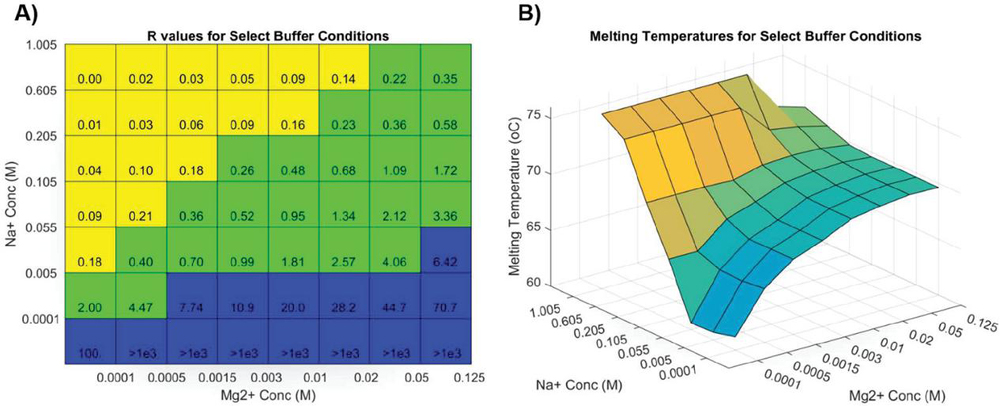
Figure 1 Simulation of Figure 8 in Owczarzy, 2008 [40] in Matlab, where oligonucleotide 5’-TGGTCTGGATCTGAGAACTTA-3’ is analyzed. A) Ion fraction R is calculated using the formula: $\sqrt{[M{g}^{2+}]}/[N{a}^{+}]$, and three parameter regimes are shown in blue, green and yellow. B) The counterion-dependent melting temperature is calculated. Reproduced from Vecchioni et al., 2018 with permission from River Publishers [41].

The behavior profile was elucidated using nonlinear fits and correction parameters that are not intuitive in the way of Allawi and SantaLucia’s nearest-neighbor model of free energy. Though highly specific, these formulas do not work for all oligos in all aqueous environments: homobase repeats, low concentrations of counterions, or the presence of other stabilizing and destabilizing molecules, modifications and substrates do not perform according to this model.

The application of both nearest-neighbor and melting temperature analyses does not extend to orthogonal base pairs: a full nearest-neighbor energy profile of the dC:Ag${+}^{}$:dC pair has not been elucidated, leading researchers to simply correct the predicted melting temperature of mismatched oligonucleotides by adding 1–2${\circ }^{}$C per metal base pair. This practice does not fully take into account metallophilic attraction between silver ions [42], which would contribute adjacency effects outside the two-body problem of nearest-neighbor calculations, though initial studies suggest that reaction favorability of a second ion is drastically reduced after a nearby ion is intercalated [43]. These factors suggests that a nearest-neighbor model may require knowledge of the opposing oligomer to allow for base pair and intercalant corrections, greatly increasing the overall number of variables and the complexity of the calculation.

1.3 Sequence Optimization Via Genetic Algorithms

Genetic algorithms (GAs) were first described by Dr. John Holland in the 1960s as an optimization tool based on observations of evolutionary biology [44]. The premise of GAs, and most optimization algorithms, involves assessing the strength, or fitness, of a particular solution to a problem. Like elementary guess-and-check methods, slight variation, or mutation, is applied to a solution. The relative fitness of the new solution is assessed, and over successive iterations, the fitness landscape is mapped to find local or global fitness maxima—the optimization algorithm seeks better answers through iteration. The primary difference between guess-and-check methods and GAs is the number of parallel solutions. Like in population biology, a set of solutions is initialized, fitness analyzed, and tournaments carried out to produce new generations of the population. In order to promote solution diversity, successful tournament winners exchange information to allow independent assortment of solution characteristics.

The linear DNA sequences in primer and nanostructure design make the analogy to living systems highly useful. Use of mutation and crossover in silico directly corresponds to natural DNA design and optimization. As such, GA tools are particularly well-suited to evolutionary optimization. The challenge to developing in silico models of DNA optimization lies in defining a fitness function that is both simple to calculate and well-suited to the design objectives. Unlike in living systems, the computational researcher does not have the luxury of hour- or yearlong generations over which to assess DNA sequence fitness. The fitness of a particular solution, or set of DNA sequences, is necessarily subject to more than one criterion, and can include: melting temperature, heterodimer size, guanine repeats, etc. There are several strategies for taking a multi-objective fitness function and producing a simple, comparison-based algorithm to assess relative fitness. The most common heuristic involves condensing the many criteria into a single numerical score based on the relative importance of the different design criteria [45]. In doing so, the various objectives are assigned variable weights, and sorted according to numerical size. A GA iterator may be designed to either maximize or minimize this fitness score, depending on the nature of the criterion.

The primary drawback of GA tools lies in this definition of this multi-objective fitness function. If there were only one criterion and a continuous fitness landscape, as in the problem: ‘minimize the distance from the square root of 200,’ there would be little trouble in attaining a highly precise near-best solution. The use of a multi-objective fitness score with weights makes the fitness landscape discontinuous: once a change occurs to increase the highest-weight criterion, solutions are boxed into one corner of the fitness landscape, preventing any true global optimization of lower-weight criteria. The fitness hill-climbing function becomes a stair-climbing function, where it is improbable that the iterator will climb back down to get around a block in the landscape. In this way, multi-objective GAs frequently find only local—rather than global—fitness maxima.

To combat the intractability of local fitness maxima, evolutionary algorithms turn to population dynamics, introducing diversity artificially. This takes the form of randomization or hypermutation, niche penalties based on population similarity, and, most importantly, gene flow. Randomization involves the formation of a small number of new solutions in a population with a much higher mutation rate than average to introduce diversity. While potentially quite useful, large tournament sizes will forcibly exclude these solutions from passing on information. Niche penalties involve increasing the global mutation rate when the overall similarity reaches a critical value. In the case of oligonucleotides, this may be assessed via the mean squared distance from the average sequence value at a particular position. Depending on the size of the steps in the fitness score, this approach may introduce diversity, or simple nudge the average solution only temporarily away from the local fitness maximum, only to return in several optimization iterations.

The two most successful approaches to diversity include elitism and gene flow. Elitism is a method that allows for greater mutation rates by saving a small number of the fittest solutions in each generation without any modification. In this way, the best solution is not lost while the general population can be subjected to higher rates of change to promote diversity. There are several methods for applying elitism, but the simplest in the context of DNA design is simply copying without mutation [45]. As in population biology, diversity can be introduced into an isolated population through the introduction of new, medium-fitness, individuals. In this way, gene flow is used to combat genetic drift, or niche creation. There are several established methods of information exchange, but all rely primarily on optimizing several independent populations and exchanging information either at distinct intervals, or after the simulation in a subsequent ‘F2 cross’ [45]. Crossing the best solutions in several populations in a follow-up simulation pits solutions clustered around distinct fitness maxima against one another, allowing for a more granular blending of characteristics at different levels in the fitness function. While there is no approach that completely fixes the diversity problem, a pointed combination of these strategies may lead to the identification of near-best solutions, given sufficient computational resources.

Several tools for primer design by GA already exist [28, 30, 46], and they rely on a multi-objective fitness function that weighs melting temperature, relative length, and dimer size between forward and reverse primer pairs. This relatively simple fitness approximation relies the primary assumption that any $\sim$20 nt primer will have only one target site in a prokaryotic or eukaryotic genome, and the calculation restricts heterodimer analysis to the primer oligonucleotides only, excluding effects of off-target dimerization on fitness calculation. This significantly speeds computation, allowing for a swift identification of primers in gene targets in the context of thousands to millions of nucleotides. Conventional DNA synthesis techniques at companies like IDT DNA are $\sim$99% efficient at adding a correct nucleotide to a growing oligo, meaning that for each nucleotide letter in an oligonucleotide sequence, there is a compounding 1% chance of an improper base. In 2019, synthesis of 25 nmol of a 20 nt primer cost $\sim$$7. Subsequent purification of the sequences via gel electrophoresis (PAGE) or liquid chromatography (HPLC) at the same company cost an additional $60. Due to the relaxed specificity needs of PCR, primers are generally not purified—99% sequence specificity over 20 nt leaves $\sim$80% primer accuracy to perform PCR (${0.99}^{20}=0.82$). Over successive amplification, defective primers remain inert. Assuming a reasonable concentration of correctly-synthesized primer, the reaction will run without oligo purification. As a result, the low cost of 20 mer oligonucleotides allows for occasional off-target dimerization, and primer failure, meaning that a computationally-efficient fitness approximation is good enough for the problem statement in PCR.

By contrast, in the case of DNA nanostructure design, any off-target dimerization will cause the failure of structural assembly. The critical regions for crossover between two adjacent helices is the 4 bp J1 junction (CAGG: CCTG), which is chosen for confirmational stability, stacking geometry, and a history of successful assembly [2, 18, 47, 48]. Any deviation from this sequence and the crossover will not occur, necessitating purification of oligos after synthesis: a lattice built with 30 mers will be unable to polymerize without removing the 27% failed product. The time and cost of purification thus makes the penalty of using a relaxed fitness calculation far more prohibitive. To mitigate this much tighter problem definition, a more robust fitness calculation and accompanying genetic algorithm toolbox are required.

As discussed, there exist a variety of tools for DNA nanotechnology design, often with an emphasis on aiding definition of sequence geometry (e.g. UNIQUMER3D [29] and caDNAno [28], industry standards). The sequence generation tools are quite relaxed, and there does not yet exist a reliable tool for specifying conserved regions of DNA, applying fitness criteria differentially across the network, or, importantly, the incorporation of orthogonal base pairing.

In this study, we present a new computational model with the goal of bridging the gap between structure topology and the sequences that exist within that framework. This model seeks to ultimately provide a generalizable, geometry-informed platform for sequence generation with diverse design criteria and base pairing environments for nucleic acid nanotechnology applications.

2 Computational Analysis of Nanostructure Composition

A de novo computational platform for DNA sequence analysis is derived and described from first principles. This platform is built from the perspective of modular nanostructure design, though it can be used in both branched and linear applications. Formulas are written to be independent of Watson-Crick parity and make note of any base pairing assumptions that are made in their derivation.

2.1 Nanostructures, Nodes and Sequences

Let M be a DNA nanostructure composed of a finite number of oligonucleotide sequences (S) where S $\in$ N${*}^{}$ for N${}^{*}=\{1,2,\mathrm{\dots }\}$, which bind together in topological units called nodes (N) for N $\in$ N${*}^{}$. M is a structure with L total base pairs, where L $\in$ N${*}^{}$, and the nodes in this network have lengths L$i_{}$ in base pairs (bp) for i $\in$ [1, N]. A network with one node is considered an unbranched duplex. By convention, in this analysis, a node is considered to be double stranded (ds), where each oligonucleotide (n$i_{}$) is bound to its logical complement (${\overline{n}}_i$) in a base pair (b$i_{}$), where b$i_{}$ $=$ [n$i_{}$:${\overline{n}}_i$], though some nodes may be single-stranded (ss) by design (N.B. a node in this context is separate from its common usage to mean “junction” in the field [49], and used in the network analysis sense to mean “distinct unit in a data structure”).

$$\begin{array}{ccccccc}\hfill 5^{\prime }-\hfill & \hfill n_1\hfill & \hfill n_2\hfill & \hfill n_3\hfill & \hfill \mathrm{\dots }\hfill & \hfill n_i\hfill & \hfill -3^{\prime }\hfill \\ & \hfill |\hfill & \hfill |\hfill & \hfill |\hfill & & \hfill |\hfill & \\ \hfill 3^{\prime }-\hfill & \hfill {\overline{n}}_1\hfill & \hfill {\overline{n}}_2\hfill & \hfill {\overline{n}}_3\hfill & \hfill \mathrm{\dots }\hfill & \hfill {\overline{n}}_i\hfill & \hfill -5^{\prime }\hfill \end{array}$$

(1)

DNA network M can be drawn conventionally using its continuous oligonucleotide sequences (Figure 2A), but can be more robustly analyzed using a nodal model (Figure 2B), where a node contains a simplex or duplex with internally consistent pairing rules, chemistry, geometry, and has connections to other nodes from its template and complement strands, and its 5’ and 3’ ends:

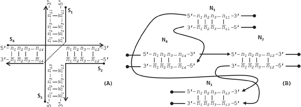
Figure 2 Representations of a Holliday junction, A) in sequence format with four sequences S$i_{}$ for for i $\in$ [1, 4], and B) in node format with four nodes N$j_{}$ for for j $\in$ [1, 4]. The primary difference between these modes of representation is that the geometry and complementarity is carried on individual nucleotides in sequence format; whereas the nature of node-based representation omits the need for complementarity indicies and just tracks the connections, or geometry, at the edges of the nodes.

Complementarity in nucleobases typically follows the binding of one purine (R) to one pyrimidine (Y) in the following set of Watson-Crick (WC) rules: { [dA:dT], [dG:dC], [rA:rU], [rG:rC] }, where dn$i_{}$ is a deoxyribonucleotide, and rn$i_{}$ is a ribonucleotide. Orthogonal base pairs can break the symmetry of WC pairing, as in the case of metal base pairs { [dC:Ag${+}^{}$:dC], [dT:Hg${2+}^{}$:dT] }. The difference in nucleobase correspondence between canonical DNA and a silver metal pairing system (CC) can be seen in the following matrix:

$$\begin{array}{cc}\hfill \mathrm{WC}\mathit{\hspace{1em}\hspace{1em}\hspace{1em}}\hfill & \hfill \mathrm{CC}\hfill \\ \hfill \begin{array}{c}\hfill dA\hfill \\ \hfill dT\hfill \\ \hfill dG\hfill \\ \hfill dC\hfill \end{array}:\left[\begin{array}{c}\hfill dT\hfill \\ \hfill dA\hfill \\ \hfill dC\hfill \\ \hfill dG\hfill \end{array}\right]\mathit{\hspace{1em}\hspace{1em}\hspace{1em}}\hfill & \hfill \begin{array}{c}\hfill dA\hfill \\ \hfill dT\hfill \\ \hfill dG\hfill \\ \hfill dC\hfill \end{array}:\left[\begin{array}{c}\hfill dT\hfill \\ \hfill dA\hfill \\ \hfill dC\hfill \\ \hfill dG,dC\hfill \end{array}\right]\hfill \end{array}$$

(2)

2.2 Heterostructures

In order to self-assemble N nodes from S oligos, analysis of nucleobase sequence must be performed to bias the energy landscape toward the desired geometry. This requires analyzing M for its heterostructures (d), or unwanted binding configurations, with length L$d_{}$. Analysis of homo- and heterodimers is carried out by aligning component strands of S or N and comparing each base in varying frames. An alignment frame (k) can be defined as the juxtaposition of two oligonucleotides, one in the 5’–3’ orientation and the other in 3’–5’ orientation, with fixed base correspondence, where k will be a frame of k${\mathit{size}}_{}$ potential base pairs. Two complementary oligonucleotides of length L$N_{}$ will form a perfect dimer of size L$d_{}$ $=$ L$N_{}$ with perfect alignment by design (see (1) above).

A homodimer is a kinetic trap for an oligonucleotide in which it is able to bind to itself in a misaligned frame, as with single-stranded oligo S$a_{}$ of length L$a_{}$ $=$ 11 nt, k${\mathit{size}}_{}$ $=$ 9 bp, L$d_{}$ $=$ 3 bp:

$$\begin{array}{cccccccccccccccccccc}\hfill 5^{\prime }-\mathrm{CA}\hfill & \hfill \mathrm{T}\hfill & \hfill \mathrm{T}\hfill & \hfill \mathrm{T}\hfill & \hfill \mathrm{G}\hfill & \hfill \mathrm{C}\hfill & \hfill \mathrm{G}\hfill & \hfill \mathrm{A}\hfill & \hfill \mathrm{A}\hfill & \hfill \mathrm{A}\hfill & \hfill -3^{\prime }\hfill & & & & & & & & & \\ & \hfill |\hfill & \hfill |\hfill & \hfill |\hfill & & & & \hfill |\hfill & \hfill |\hfill & \hfill |\hfill & & & & & & & & & & \\ \hfill 3^{\prime }-\hfill & \hfill \mathrm{A}\hfill & \hfill \mathrm{A}\hfill & \hfill \mathrm{A}\hfill & \hfill \mathrm{G}\hfill & \hfill \mathrm{C}\hfill & \hfill \mathrm{G}\hfill & \hfill \mathrm{T}\hfill & \hfill \mathrm{T}\hfill & \hfill \mathrm{T}\hfill & \hfill \mathrm{AC}\hfill & \hfill -5^{\prime }\hfill & & & & & & & & \end{array}$$

(3)

A heterodimer can be defined as the inappropriate binding of two disparate oligonucleotides, as with single-stranded oligos S$b_{}$ and S$c_{}$ of lengths L$b_{}$ $=$ 11 nt, L$c_{}$ $=$ 14 nt, k${\mathit{size}}_{}$ $=$ 11 bp, and L$d_{}$ $=$ 7 bp:

$$\begin{array}{cccccccccccccccccccc}\hfill 5^{\prime }-\hfill & \hfill \mathrm{A}\hfill & \hfill \mathrm{T}\hfill & \hfill \mathrm{A}\hfill & \hfill \mathrm{T}\hfill & \hfill \mathrm{A}\hfill & \hfill \mathrm{T}\hfill & \hfill \mathrm{C}\hfill & \hfill \mathrm{GCCG}-3^{\prime }\hfill & & & & & & & & & & & \\ & \hfill |\hfill & \hfill |\hfill & \hfill |\hfill & \hfill |\hfill & \hfill |\hfill & \hfill |\hfill & \hfill |\hfill & & & & & & & & & & & & \\ \hfill 3^{\prime }-\mathrm{CT}\hfill & \hfill \mathrm{T}\hfill & \hfill \mathrm{A}\hfill & \hfill \mathrm{T}\hfill & \hfill \mathrm{A}\hfill & \hfill \mathrm{T}\hfill & \hfill \mathrm{A}\hfill & \hfill \mathrm{G}\hfill & \hfill \mathrm{GTAGA}-5^{\prime }\hfill & & & & & & & & & & & \end{array}$$

(4)

Detailed analysis of alignment and indexing for dimer analysis can be found in Appendix A.

2.3 Other Sequence Design Criteria

In addition to dimer size minimization, DNA nanostructure design requires the minimization of other types of criteria as a result of thermodynamic or design-related criteria. All of the following analyses can be carried out using the single strand indexing rules found in Tables 3–4. Because they pertain to the presence of consecutive sequence elements, the rules described do not need to be subjected to repetition through slip and frame alignment, as with homo- and heterodimer search algorithms.

2.3.1 Gap analysis: ‘gapN’

To utilize the emergent electrical characteristics of nucleotide pairing, defining, a resistor (WC pairing), a conductor (dC:Ag${+}^{}$:dC pairing) [50], or a semiconductor (guanine tetraplex formation) [51], it is most likely necessary to maximize density of a particular pairing regime across a polymerized oligonucleotide. Criteria such as gate analysis, which sets a percent occupancy for a particular nucleotide, may lead to unintended clustering of the preferred nucleotide at one end of the sequence, as with 75% guanine sequence: 5’-GGGGGGGGGATA-3’. While guanine may have the lowest base ionization energy of the four WC nucleotides [52], an AT 3mer will interfere with the proposed conductance pathway. Gate criteria are thus useful for applications such as primer design, where GC occupancy is analyzed in percentages. For nanowire design, we instead introduce gap criteria, in which the maximum distance between a target base pair, not nucleobase, is tracked and minimized. Take for instance the sequence in (B.2.c Comparison of fragmented and single-node networks) below where AT gap analysis is tracked and set to a maximum of 1 base pair.

$$\begin{array}{ccccccccccccc}\hfill 5^{\prime }-\hfill & \hfill \mathrm{A}\hfill & \hfill \mathrm{T}\hfill & \hfill \mathrm{A}\hfill & \hfill \mathrm{T}\hfill & \hfill \mathrm{A}\hfill & \hfill \mathrm{T}\hfill & \hfill \mathbf{\text{C}}\hfill & \hfill \mathrm{A}\hfill & \hfill \mathrm{A}\hfill & \hfill \mathbf{\text{G}}\hfill & \hfill \mathrm{T}\hfill & \hfill -3^{\prime }\hfill \\ & \hfill |\hfill & \hfill |\hfill & \hfill |\hfill & \hfill |\hfill & \hfill |\hfill & \hfill |\hfill & \hfill |\hfill & \hfill |\hfill & \hfill |\hfill & \hfill |\hfill & \hfill |\hfill & \\ \hfill 3^{\prime }-\hfill & \hfill \mathrm{T}\hfill & \hfill \mathrm{A}\hfill & \hfill \mathrm{T}\hfill & \hfill \mathrm{A}\hfill & \hfill \mathrm{T}\hfill & \hfill \mathrm{A}\hfill & \hfill \mathbf{\text{G}}\hfill & \hfill \mathrm{T}\hfill & \hfill \mathrm{T}\hfill & \hfill \mathbf{\text{C}}\hfill & \hfill \mathrm{A}\hfill & \hfill -5^{\prime }\hfill \end{array}$$

(5)

Gap analysis on this sequence shows the presence of 2 gaps in the AT occupancy, each of size 1 bp. Note the equvalence between dA:dT and dT:dA. The following sequence (60) instead fails the ‘gap1’ criterion for the AT base pair:

$$\begin{array}{ccccccccccccc}\hfill 5^{\prime }-\hfill & \hfill \mathrm{A}\hfill & \hfill \mathrm{T}\hfill & \hfill \mathrm{A}\hfill & \hfill \mathrm{T}\hfill & \hfill \mathrm{A}\hfill & \hfill \mathbf{\text{C}}\hfill & \hfill \mathbf{\text{C}}\hfill & \hfill \mathrm{A}\hfill & \hfill \mathrm{A}\hfill & \hfill \mathbf{\text{G}}\hfill & \hfill \mathrm{T}\hfill & \hfill -3^{\prime }\hfill \\ & \hfill |\hfill & \hfill |\hfill & \hfill |\hfill & \hfill |\hfill & \hfill |\hfill & \hfill |\hfill & \hfill |\hfill & \hfill |\hfill & \hfill |\hfill & \hfill |\hfill & \hfill |\hfill & \\ \hfill 3^{\prime }-\hfill & \hfill \mathrm{T}\hfill & \hfill \mathrm{A}\hfill & \hfill \mathrm{T}\hfill & \hfill \mathrm{A}\hfill & \hfill \mathrm{T}\hfill & \hfill \mathbf{\text{G}}\hfill & \hfill \mathbf{\text{G}}\hfill & \hfill \mathrm{T}\hfill & \hfill \mathrm{T}\hfill & \hfill \mathbf{\text{C}}\hfill & \hfill \mathrm{A}\hfill & \hfill -5^{\prime }\hfill \end{array}$$

(6)

Two gaps are identified, the first [dCdC:dGdG], and the second [dG:dC]. Highlighted in red is the size 2 bp gap that violates the prescribed ‘gap1’ rule. We can again perform the same ‘gap1’ analysis for CC pairing (dC:Ag${+}^{}$:dC):

$$\begin{array}{ccccccccccccc}\hfill 5^{\prime }-\hfill & \hfill \mathrm{C}\hfill & \hfill \mathrm{C}\hfill & \hfill \mathbf{\text{A}}\hfill & \hfill \mathrm{C}\hfill & \hfill \mathbf{\text{C}}\hfill & \hfill \mathrm{C}\hfill & \hfill \mathrm{C}\hfill & \hfill \mathbf{\text{A}}\hfill & \hfill \mathrm{C}\hfill & \hfill \mathbf{\text{C}}\hfill & \hfill \mathbf{\text{T}}\hfill & \hfill -3^{\prime }\hfill \\ & \hfill \bullet \hfill & \hfill \bullet \hfill & \hfill |\hfill & \hfill \bullet \hfill & \hfill |\hfill & \hfill \bullet \hfill & \hfill \bullet \hfill & \hfill |\hfill & \hfill \bullet \hfill & \hfill \bullet \hfill & \hfill |\hfill & \\ \hfill 3^{\prime }-\hfill & \hfill \mathrm{C}\hfill & \hfill \mathrm{C}\hfill & \hfill \mathbf{\text{T}}\hfill & \hfill \mathrm{C}\hfill & \hfill \mathbf{\text{G}}\hfill & \hfill \mathrm{C}\hfill & \hfill \mathrm{C}\hfill & \hfill \mathbf{\text{T}}\hfill & \hfill \mathrm{C}\hfill & \hfill \mathrm{C}\hfill & \hfill \mathbf{\text{A}}\hfill & \hfill -5^{\prime }\hfill \end{array}$$

(7)

In (7), the sequence presents 3 size 1 bp gaps (bold) in the CC paired nanowire, passing analysis for ‘gap1’ consideration. Note that the cytosine base in [dC:dG] does not evade detection as it is not paired to an opposing cytosine nucleobase, and it therefore counts toward a CC sequence gap. In contrast, the following sequence will fail ‘gap1’ analysis:

$$\begin{array}{ccccccccccccc}\hfill 5^{\prime }-\hfill & \hfill \mathrm{C}\hfill & \hfill \mathrm{C}\hfill & \hfill \mathbf{\text{A}}\hfill & \hfill \mathrm{C}\hfill & \hfill \mathbf{\text{A}}\hfill & \hfill \mathbf{\text{C}}\hfill & \hfill \mathrm{C}\hfill & \hfill \mathbf{\text{A}}\hfill & \hfill \mathrm{C}\hfill & \hfill \mathbf{\text{C}}\hfill & \hfill \mathbf{\text{T}}\hfill & \hfill -3^{\prime }\hfill \\ & \hfill \bullet \hfill & \hfill \bullet \hfill & \hfill |\hfill & \hfill \bullet \hfill & \hfill |\hfill & \hfill \bullet \hfill & \hfill \bullet \hfill & \hfill |\hfill & \hfill \bullet \hfill & \hfill \bullet \hfill & \hfill |\hfill & \\ \hfill 3^{\prime }-\hfill & \hfill \mathrm{C}\hfill & \hfill \mathrm{C}\hfill & \hfill \mathbf{\text{T}}\hfill & \hfill \mathrm{C}\hfill & \hfill \mathbf{\text{T}}\hfill & \hfill \mathbf{\text{G}}\hfill & \hfill \mathrm{C}\hfill & \hfill \mathbf{\text{T}}\hfill & \hfill \mathrm{C}\hfill & \hfill \mathrm{C}\hfill & \hfill \mathbf{\text{A}}\hfill & \hfill -5^{\prime }\hfill \end{array}$$

(8)

In (8), the presence of the [dAdC:dGdT] subsequence acts as a size 2 bp CC gap (red), failing ‘gap1’ analysis, but passing ‘gap2’ analysis. To design dC:Ag${+}^{}$:dC nanowires with reasonable molecular conductance, we apply a ‘gap1’ CC rule to force any region that is conductive by design to have at most one non-metallic base pair in a row.

2.3.2 Purines and pyrimidines: ‘R4’ and ‘Y4’

The overabundance of consecutive purines or pyrimidines in single oligonucleotides may affect the twist of the double helix through abnormal stacking interactions. To maintain predictable rotational dynamics within a structure, allowing the formation of predictable geometry, it is conventional to restrict the total number of consecutive purines (‘R’ $=$ A,G) and pyrimidines (‘Y’ $=$ C,T) to four. Note that unlike gapping, this tracking occurs on single nucleotides, not base pairs, generating parallel analyses for each half of the node. An example of ‘Y4’ analysis is shown in (63):

$$\begin{array}{ccccccccccccc}\hfill 5^{\prime }-\hfill & \hfill \mathbf{\text{C}}\hfill & \hfill \mathbf{\text{C}}\hfill & \hfill \mathrm{A}\hfill & \hfill \mathbf{\text{C}}\hfill & \hfill \mathbf{\text{T}}\hfill & \hfill \mathbf{\text{C}}\hfill & \hfill \mathbf{\text{C}}\hfill & \hfill \mathbf{\text{T}}\hfill & \hfill \mathbf{\text{C}}\hfill & \hfill \mathbf{\text{C}}\hfill & \hfill \mathbf{\text{T}}\hfill & \hfill -3^{\prime }\hfill \\ & \hfill \bullet \hfill & \hfill \bullet \hfill & \hfill |\hfill & \hfill \bullet \hfill & \hfill |\hfill & \hfill \bullet \hfill & \hfill \bullet \hfill & \hfill |\hfill & \hfill \bullet \hfill & \hfill \bullet \hfill & \hfill |\hfill & \\ \hfill 3^{\prime }-\hfill & \hfill \mathrm{C}\hfill & \hfill \mathrm{C}\hfill & \hfill \mathbf{\text{T}}\hfill & \hfill \mathbf{\text{C}}\hfill & \hfill \mathbf{\text{A}}\hfill & \hfill \mathrm{G}\hfill & \hfill \mathbf{\text{C}}\hfill & \hfill \mathrm{A}\hfill & \hfill \mathbf{\text{C}}\hfill & \hfill \mathbf{\text{C}}\hfill & \hfill \mathbf{\text{A}}\hfill & \hfill -5^{\prime }\hfill \end{array}$$

(9)

Here the top sequence presents a pyrimidine 8mer (red) as well as a 2mer (bold). The bottom strand presents a 4mer, a 2mer and a 1mer (bold). The top sequence will fail ‘Y4’ analysis. In contrast, the following duplex shows ‘R4’ analysis:

$$\begin{array}{ccccccccccccc}\hfill 5^{\prime }-\hfill & \hfill \mathrm{C}\hfill & \hfill \mathrm{C}\hfill & \hfill \mathbf{\text{A}}\hfill & \hfill \mathrm{C}\hfill & \hfill \mathrm{T}\hfill & \hfill \mathrm{C}\hfill & \hfill \mathrm{C}\hfill & \hfill \mathrm{T}\hfill & \hfill \mathrm{C}\hfill & \hfill \mathrm{C}\hfill & \hfill \mathrm{T}\hfill & \hfill -3^{\prime }\hfill \\ & \hfill \bullet \hfill & \hfill \bullet \hfill & \hfill |\hfill & \hfill \bullet \hfill & \hfill |\hfill & \hfill \bullet \hfill & \hfill \bullet \hfill & \hfill |\hfill & \hfill \bullet \hfill & \hfill \bullet \hfill & \hfill |\hfill & \\ \hfill 3^{\prime }-\hfill & \hfill \mathrm{C}\hfill & \hfill \mathrm{C}\hfill & \hfill \mathrm{T}\hfill & \hfill \mathrm{C}\hfill & \hfill \mathbf{\text{A}}\hfill & \hfill \mathbf{\text{G}}\hfill & \hfill \mathbf{\text{G}}\hfill & \hfill \mathbf{\text{A}}\hfill & \hfill \mathbf{\text{G}}\hfill & \hfill \mathrm{C}\hfill & \hfill \mathbf{\text{A}}\hfill & \hfill -5^{\prime }\hfill \end{array}$$

(10)

The top sequence passes purine analysis (though it has 8 consecutive pyrimidines), while the bottom strand presents 5 consecutive purines [dAdGdGdAdG] (red) and summarily fails the ‘R4’ criterion. Because of C:C pairing, neither (9) nor (10) have symmetrical purine and pyrimidine analysis. In WC conditions, all purine repeats will pair with pyrimidine repeats of equal size within the same node.

2.3.3 GC/AT: ‘S4’/‘W4’

For similar reasons, it is customary to minimize the number of consecutive C:G and A:T pairs to 4 bp. By convention, C:G pair are abbreviated as ‘strong’ (S) owing to their three hydrogen bonds, while A:T bonds are abbreviated as ‘weak’ (W) for containing two hydrogen bonds. Because currently known metal base pairs are homobase dimers, both strands in a duplexed node will achieve the same fitness score:

$$\begin{array}{ccccccccccccc}\hfill 5^{\prime }-\hfill & \hfill \mathbf{\text{A}}\hfill & \hfill \mathbf{\text{T}}\hfill & \hfill \mathbf{\text{A}}\hfill & \hfill \mathbf{\text{T}}\hfill & \hfill \mathbf{\text{A}}\hfill & \hfill \mathrm{C}\hfill & \hfill \mathrm{C}\hfill & \hfill \mathbf{\text{A}}\hfill & \hfill \mathbf{\text{A}}\hfill & \hfill \mathrm{G}\hfill & \hfill \mathbf{\text{T}}\hfill & \hfill -3^{\prime }\hfill \\ & \hfill |\hfill & \hfill \bullet \hfill & \hfill |\hfill & \hfill |\hfill & \hfill |\hfill & \hfill |\hfill & \hfill |\hfill & \hfill |\hfill & \hfill |\hfill & \hfill |\hfill & \hfill |\hfill & \\ \hfill 3^{\prime }-\hfill & \hfill \mathbf{\text{T}}\hfill & \hfill \mathbf{\text{T}}\hfill & \hfill \mathbf{\text{T}}\hfill & \hfill \mathbf{\text{A}}\hfill & \hfill \mathbf{\text{T}}\hfill & \hfill \mathrm{G}\hfill & \hfill \mathrm{G}\hfill & \hfill \mathbf{\text{T}}\hfill & \hfill \mathbf{\text{T}}\hfill & \hfill \mathrm{C}\hfill & \hfill \mathbf{\text{A}}\hfill & \hfill -5^{\prime }\hfill \end{array}$$

(11)

In (65), the sequence presents 5mer, 2mer and 1mer weak pair repeats, which fails the ‘W4’ design criterion, even with a dT:Hg${2+}^{}$:dT base pair. By contrast, the C:C bonding sequence in (66) will symmetrically fail ‘S4’ analysis:

$$\begin{array}{ccccccccccccc}\hfill 5^{\prime }-\hfill & \hfill \mathbf{\text{C}}\hfill & \hfill \mathbf{\text{C}}\hfill & \hfill \mathrm{A}\hfill & \hfill \mathbf{\text{C}}\hfill & \hfill \mathrm{A}\hfill & \hfill \mathbf{\text{C}}\hfill & \hfill \mathbf{\text{C}}\hfill & \hfill \mathbf{\text{G}}\hfill & \hfill \mathbf{\text{C}}\hfill & \hfill \mathbf{\text{C}}\hfill & \hfill \mathrm{T}\hfill & \hfill -3^{\prime }\hfill \\ & \hfill \bullet \hfill & \hfill \bullet \hfill & \hfill |\hfill & \hfill \bullet \hfill & \hfill |\hfill & \hfill |\hfill & \hfill \bullet \hfill & \hfill |\hfill & \hfill \bullet \hfill & \hfill \bullet \hfill & \hfill \mathbf{|}\hfill & \\ \hfill 3^{\prime }-\hfill & \hfill \mathbf{\text{C}}\hfill & \hfill \mathbf{\text{C}}\hfill & \hfill \mathrm{T}\hfill & \hfill \mathbf{\text{C}}\hfill & \hfill \mathrm{T}\hfill & \hfill \mathbf{\text{G}}\hfill & \hfill \mathbf{\text{C}}\hfill & \hfill \mathbf{\text{C}}\hfill & \hfill \mathbf{\text{C}}\hfill & \hfill \mathbf{\text{C}}\hfill & \hfill \mathbf{\text{A}}\hfill & \hfill -5^{\prime }\hfill \end{array}$$

(12)

Here, both the top and bottom strands present strong base pair repeats of sizes 5 (red), 2 and 1 nt (bold), regardless of ion distribution. The symmetry of this fitness criterion is immune to homobase orthogonal base pairs.

In practice, the W4 criterion may be relaxed to accommodate other design parameters.

2.3.4 Guanine repeats: ‘G3’

The overexpression of guanine in an oligonucleotide may lead to the formation of a guanine tetraplex. To avoid kinetic traps or unintended geometries associated with tetraplex formation, we restrict the number of consecutive guanines to 3 nt, applying a ‘G3’ cap on single stranded sequences. This rule is not symmetrical, and the fitness score does not carry over from template to complement.

$$\begin{array}{ccccccccccccc}\hfill 5^{\prime }-\hfill & \hfill \mathbf{\text{G}}\hfill & \hfill \mathbf{\text{G}}\hfill & \hfill \mathrm{C}\hfill & \hfill \mathrm{T}\hfill & \hfill \mathrm{C}\hfill & \hfill \mathrm{C}\hfill & \hfill \mathrm{C}\hfill & \hfill \mathrm{C}\hfill & \hfill \mathrm{A}\hfill & \hfill \mathbf{\text{G}}\hfill & \hfill \mathrm{T}\hfill & \hfill -3^{\prime }\hfill \\ & \hfill |\hfill & \hfill |\hfill & \hfill |\hfill & \hfill |\hfill & \hfill |\hfill & \hfill |\hfill & \hfill |\hfill & \hfill |\hfill & \hfill |\hfill & \hfill |\hfill & \hfill |\hfill & \\ \hfill 3^{\prime }-\hfill & \hfill \mathrm{C}\hfill & \hfill \mathrm{C}\hfill & \hfill \mathbf{\text{G}}\hfill & \hfill \mathrm{A}\hfill & \hfill \mathbf{\text{G}}\hfill & \hfill \mathbf{\text{G}}\hfill & \hfill \mathbf{\text{G}}\hfill & \hfill \mathbf{\text{G}}\hfill & \hfill \mathrm{T}\hfill & \hfill \mathrm{C}\hfill & \hfill \mathrm{A}\hfill & \hfill -5^{\prime }\hfill \end{array}$$

(13)

The duplex shown in (67) will fail ‘G3’ analysis, as the bottom sequence has a guanine 4mer (red). The largest guanine repeat in the top sequence is 2 nt (bold). To fix a sequence with this design, we can consider switching one [dC:dG] pair for a [dG:dC] pair.

3 Computational Design of Nanostructures using a Genetic Algorithm

Using the computational framework established above, we outline the design and construction of a genetic algorithm toolbox in Matlab for branched, orthogonal DNA sequence design.

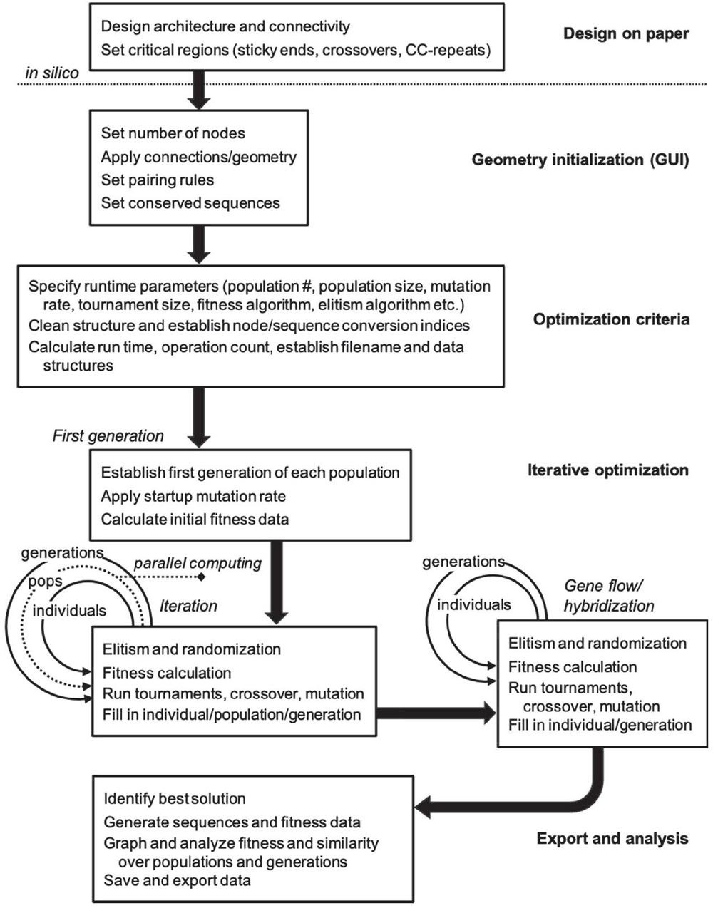
Figure 3 Process workflow for nanostructure sequence design algorithm.

3.1 Generic Workflow

The algorithm follows a general GA workflow with initialization and iteration phases. Design of topology and conserved regions occurs on paper and in other software packages. Within this toolbox there are three distinct phases of operation. In the first phase, optimization and iteration criteria are defined precisely through graphical user interface (GUI) and .m file entry. In the second phase, the model is then initialized, and data structures are pre-allocated based on user specifications. Parallel iteration begins in separate population files, and a subsequent F2 cross between best solutions is carried out. In the final phase, runtime analysis is performed, sequence data are stored, and graphical data are exported for the user. A diagrammatic explanation of this information can be found in Figure 3.

3.2 Nanostructure Optimization

Detailed implementation of the genetic algorithm can be found in Appendix D. The main optimization occurs through fitness calculation for a population of solutions. Detailed fitness calculation and weight can be found in the Appendix. In brief, the criteria described in Appendix D are implemented in a weighted sum, with dimers of size 8 evaluated to be of equal penalty to repeats (Y3, R3, etc.) of size 3. This balance can be manually specified in the running of the algorithm. Evaluation of runtime statistics and fitness tracking is discussed.

4 Experimental Validation: Algorithmic Design of a Non-canonical DNA Nanostructure

4.1 Nanostructure Design Frame

To validate our genetic algorithm, we modified a well-characterized DNA nanostructure to robustly assemble with environmental Ag${+}^{}$. As a test case, we utilized one of the Double crossover motifs, the DAO molecule, which was first described in 1998, and is characterized by two Antiparallel double helical segments of 32 bp with two crossovers spaced an Odd number of half turns apart (16 bp) [18]. In this experiment, junction sequences were altered to include a C:C spacer between the adjacent helices (nodes N${\mathrm{19}}_{}$ and N${\mathrm{20}}_{}$, Figure 4). This modification is slight enough to allow the overall topology to be retained but provides an impetus for non-canonical sequence optimization to account for off-target dimerization in the presence of Ag${+}^{}$.

Figure 4 Template for modification of the DAO tile with C-Ag${+}^{}$-C bonds. The four sequences (S$X_{}$) are marked as well as the twenty nodes for computational design (N$X_{}$). Design considerations at each point are marked. On the external frame bold black lines indicate template strands, while thin black dotted lines indicate complements. Directionality (5$\prime$ to 3$\prime$) is indicated by arrows. Conserved sequences are indicated by letters (G,T,A,C), while nucleotides that are optimized computationally are denoted with a colored dash (‘—’).

4.2 Computational Modeling

Twenty nodes were initialized into the GA with varying criteria. Junction nodes (N${\mathrm{3}}_{}$, N${\mathrm{4}}_{}$, N${\mathrm{6}}_{}$, N${\mathrm{7}}_{}$, N${\mathrm{12}}_{}$, N${\mathrm{13}}_{}$, N${\mathrm{15}}_{}$, N${\mathrm{16}}_{}$) were left unmodified from the original motif and set to uneditable. Terminal nodes (N${\mathrm{1}}_{}$, N${\mathrm{9}}_{}$, N${\mathrm{10}}_{}$, N${\mathrm{18}}_{}$) have a GC gap applied to force a strong pair at that position. The C-Ag${+}^{}$-C crossover nodes (N${\mathrm{19}}_{}$, N${\mathrm{20}}_{}$) were set to CC-parity and left uneditable. In this way, the bulk of optimization was carried out on the duplex nodes (N${\mathrm{2}}_{}$, N${\mathrm{5}}_{}$, N${\mathrm{8}}_{}$, N${\mathrm{11}}_{}$, N${\mathrm{14}}_{}$, N${\mathrm{17}}_{}$, as well as restrained N${\mathrm{1}}_{}$, N${\mathrm{9}}_{}$, N${\mathrm{10}}_{}$, N${\mathrm{18}}_{}$) to optimize sequences that balanced the diverse design criteria of the overall nanostructure. Standard runtime parameters were utilized: 10 solution populations of size 40, a mutation rate of 5%, and a simulation time of 500 generations. In Appendix D, Figure 21 shows the fitness scores of populations in this simulation, while Figures 22–24 are representative of shorter simulation times on this frame (100 generations). Model-generated sequences can be found in Table 1, while the dimerization and repeat statistics can be seen in Table 2. The final motif is shown in Figure 5.

Table 1 DAO-CCxover tile sequences (CC bold)

Sequence #	Nucleotide Sequence
DAO-CCx-S1	5’-GTAACACACCCAGATAG-3’
DAO-CCx-S2	5’-CTATCTGGACTAAGTAGACAATCACCC
	AAACTATGACATCCTGTGTTAC-3’
DAO-CCx-S3	5’-GTGAATCCTGATTGTCTACTTAGTCGG
	ATGTCATAGTTTGGACTTGTTG-3’
DAO-CCx-S4	5’-CAACAAGTCGGATTCAC-3’

Table 2 DAO-CCxover modeling results

Histogram Bins for n-mers	1-mers	2-mers	3-mers	4-mers	5-mers
Dimers	1630	518	168	44	5
Purine repeats	18	8	10
Pyrimidine repeats	16	10	8	2
AT repeats	18	8	14
GC repeats	36	4	4
Guanine repeats	18	4

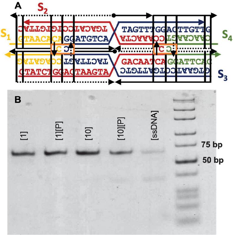
Figure 5 DAO-CCxover motif. (A) Model-generated sequences are shown on the design frame. (B) Nondenaturing 6% PAGE shows the successful assembly of the motif (64 bp) with stoichiometric [1] or 10-fold excess [10] AgNO$3_{}$. Precipitation of environmental Ag+ by adding NaCl to 50 mM [P] does not perturb the motif. Single stranded DNA without annealing is shown for contrast.

4.3 Experimental Results

The four sequences in Table 1 were purchased from IDT DNA (Coralville, IO, USA) with denaturing polyacrylamide gel electrophoresis (PAGE) purification. Annealing was carried out at 2 uM DNA in 10 mM MOPS with 12.5 mM MgSO$4_{}$ and 100 mM NaNO$3_{}$ at pH 7.7 by heating a water bath to 95${\circ }^{}$C and slowly cooling to room temperature over 48 hours. Resulting structures were visualized by 6% native PAGE and stained with StainsAll (Sigma-Aldrich, St. Louis, MO, USA). Precipitation of environmental Ag${+}^{}$ after annealing was carried out as described previously [41], by adding NaCl to 50 mM and extracting supernatant after sedimentation. This process was repeated three times.

The gel results show that the DAO variant assembles reliably into a single band after stoichiometric annealing of oligos and ions. Precipitation of the Ag${+}^{}$ does not disrupt the motif, except in the case of 10-fold excess Ag${+}^{}$, where some single-stranded oligos are visualized. The applications of this structure are beyond the scope of this manuscript, but it is clear that sequences generated by our genetic algorithm perform well, annealing into the desired motif in the presence of Ag${+}^{}$.

5 Conclusions

We present a novel computational model grounded upon ab initio calculations on DNA networks. We demonstrate that nucleic acid secondary structures can be broken into a set of linearly-independent nodes and edges, and that these networks are amenable to analysis through careful sequence alignment. By employing reverse indexing schemes and operation count optimization, we are able to efficiently scan large networks in an iterative framework. The fracturing of a nanostructure into component nodes allows for the assignation of diverse sequence design criteria, in which we are able to apply diverse parity schemes, junction sequences, sticky ends, and nucleobase gap criteria in a modular fashion. After parametrization of these DNA networks, we build and employ a genetic algorithm for the optimization of large solution pools, and we employ population dynamics and parallel computing to overcome local fitness maxima and provide more globally-optimized nucleic acid sequences.

To validate our model, we modified a canonical DNA motif, the DAO molecule, to contain two C:Ag${+}^{}$:C base pairs, and further optimized the sequence to be resistant to off-target dimerization driven by the presence of Ag${+}^{}$. This algorithmically-generated motif assembled efficiently, underscoring the utility of our computational framework. In this manner, we have solved the sequence design problem for metal-mediated and other orthogonal base pairing regimes through the use of a modular genetic algorithm. This model may be used to subsequently probe the topological implications of parity modifications by providing robust oligomeric sequences for challenging design environments.

Acknowledgements

We gratefully acknowledge support by National Space Technology Research Grant NNX14AM51H to SV, LJR, and SJW. This work was partially supported by the US National Science Foundation via grant 1662329 to SV. RS and NCS were supported by DE-SC0007991 from the Department of Energy and CCF-2106790 from the National Science Foundation.

Data Availability

Code and supporting data are available upon request to sv1091@nyu.edu.

Appendix A: Algorithmic Analysis of Heterodimers using Frame Alignment

A.1 Oligonucleotide Slip

Testing for inappropriate heterostructures requires comparison of nucleotides with different alignment frames, in which ’slip’ can be defined as the size of the 5’ or 3’ overhang of the first sequence. Slip can be visualized in the following manner:

$$\begin{array}{cccccccccccccccc}& \hfill 5^{\prime }-\hfill & \hfill \mathrm{A}\hfill & \hfill \mathrm{T}\hfill & \hfill \mathrm{A}\hfill & \hfill \mathrm{T}\hfill & \hfill \mathrm{A}\hfill & \hfill \mathrm{T}\hfill & \hfill \mathrm{C}\hfill & \hfill \mathrm{G}\hfill & \hfill \mathrm{CCG}-3^{\prime }\hfill & & & & & \\ & & \hfill |\hfill & \hfill |\hfill & \hfill |\hfill & \hfill |\hfill & \hfill |\hfill & \hfill |\hfill & \hfill |\hfill & & & & & & & \\ \hfill 3^{\prime }-\hfill & \hfill \mathbf{\text{C}}\mathbf{\text{T}}\hfill & \hfill \mathrm{T}\hfill & \hfill \mathrm{A}\hfill & \hfill \mathrm{T}\hfill & \hfill \mathrm{A}\hfill & \hfill \mathrm{T}\hfill & \hfill \mathrm{A}\hfill & \hfill \mathrm{G}\hfill & \hfill \mathrm{G}\hfill & \hfill \mathrm{TAGA}-5^{\prime }\hfill & & & & & \end{array}$$

(14)

$$\begin{array}{cccccccccccccccccccc}\hfill 5^{\prime }-\mathbf{\text{TCA}}& \hfill \mathrm{T}\hfill & \hfill \mathrm{T}\hfill & \hfill \mathrm{T}\hfill & \hfill \mathrm{G}\hfill & \hfill \mathrm{C}\hfill & \hfill \mathrm{G}\hfill & \hfill \mathrm{A}\hfill & \hfill \mathrm{A}\hfill & \hfill \mathrm{A}\hfill & \hfill -3^{\prime }\hfill & & & & & & & & & \\ & \hfill |\hfill & \hfill |\hfill & \hfill |\hfill & & & & \hfill |\hfill & \hfill |\hfill & \hfill |\hfill & & & & & & & & & & \\ \hfill 3^{\prime }-& \hfill \mathrm{A}\hfill & \hfill \mathrm{A}\hfill & \hfill \mathrm{A}\hfill & \hfill \mathrm{G}\hfill & \hfill \mathrm{C}\hfill & \hfill \mathrm{G}\hfill & \hfill \mathrm{T}\hfill & \hfill \mathrm{T}\hfill & \hfill \mathrm{T}\hfill & \hfill \mathrm{AC}-5^{\prime }\hfill & & & & & & & & & \end{array}$$

(15)

Scheme (14) shows the top strand slipping to the right two nucleotides relative to alignment, while (15) the top strand slipping to the left three nucleotides. These two slip conditions can be called forward slip and backward slip (s$f_{}$ and s$b_{}$), respectively. The case where two strands are aligned in the correct frame can be called a special case of forward slip, where $s_f=0$. To avoid repeat comparison, the case where $s_b=0$ is disallowed. A general formula for slip can be derived from the following example, where two sequences (S$a_{}$, S$b_{}$) with unequal lengths ($L_a=5$ nt, $L_b=3$ nt) are aligned in all possible frames:

$$\begin{array}{c}\hfill {\mathit{s}}_{\mathit{f}}=\mathbf{\text{0}}\hfill \\ \hfill \begin{array}{ccccc}\hfill 5^{\prime }-\hfill & \hfill n_1\hfill & \hfill n_2\hfill & \hfill n_3\hfill & n_4-3^{\prime }\hfill \\ & \hfill |\hfill & \hfill |\hfill & \hfill |\hfill & \\ \hfill 3^{\prime }-\hfill & \hfill n_5\hfill & \hfill n_6\hfill & \hfill n_7\hfill & -5^{\prime }\hfill \end{array}\hfill \end{array}\mathit{\hspace{1em}}\begin{array}{c}\hfill {\mathit{s}}_{\mathit{f}}=\mathbf{\text{1}}\hfill \\ \hfill \begin{array}{ccccc}\hfill 5^{\prime }-& \hfill n_1\hfill & \hfill n_2\hfill & \hfill n_3\hfill & n_4-3^{\prime }\hfill \\ & \hfill |\hfill & \hfill |\hfill & & \\ \hfill 3^{\prime }-n_5& \hfill n_6\hfill & \hfill n_7\hfill & \hfill -5^{\prime }\hfill & \end{array}\hfill \end{array}$$
$$\begin{array}{c}\hfill {\mathit{s}}_{\mathit{f}}=\mathbf{\text{2}}\hfill \\ \hfill \begin{array}{ccccc}\hfill 5^{\prime }-& \hfill n_1\hfill & \hfill n_2\hfill & \hfill n_3\hfill & n_4-3^{\prime }\hfill \\ & \hfill |\hfill & & & \\ \hfill 3^{\prime }-n_5{n}_6& \hfill n_7\hfill & \hfill -5^{\prime }\hfill & & \end{array}\hfill \end{array}$$
$$\begin{array}{c}\hfill {\mathit{s}}_{\mathit{b}}=\mathbf{\text{1}}\hfill \\ \hfill \begin{array}{ccccc}\hfill 5^{\prime }-n_1& \hfill n_2\hfill & \hfill n_3\hfill & \hfill n_4\hfill & -3^{\prime }\hfill \\ & \hfill |\hfill & \hfill |\hfill & \hfill |\hfill & \\ \hfill 3^{\prime }-& \hfill n_5\hfill & \hfill n_6\hfill & \hfill n_7\hfill & -5^{\prime }\hfill \end{array}\hfill \end{array}\mathit{\hspace{1em}}\begin{array}{c}\hfill {\mathit{s}}_{\mathit{b}}=\mathbf{\text{2}}\hfill \\ \hfill \begin{array}{cccc}\hfill 5^{\prime }-n_1{n}_2& \hfill n_3\hfill & \hfill n_4\hfill & -3^{\prime }\hfill \\ & \hfill |\hfill & \hfill |\hfill & \\ \hfill 3^{\prime }-& \hfill n_5\hfill & \hfill n_6\hfill & n_7-5^{\prime }\hfill \end{array}\hfill \end{array}$$
$$\begin{array}{c}\hfill {\mathit{s}}_{\mathit{b}}=\mathbf{\text{3}}\hfill \\ \hfill \begin{array}{ccc}\hfill 5^{\prime }-n_1{n}_2{n}_3& \hfill n_4\hfill & -3^{\prime }\hfill \\ & \hfill |\hfill & \\ \hfill 3^{\prime }-& \hfill n_5\hfill & n_6{n}_7-5^{\prime }\hfill \end{array}\hfill \end{array}$$	(16)

Forward slip begins with frame alignment and proceeds until the first nucleotide in S$a_{}$ (5’–3’) corresponds to the last nucleotide in S$b_{}$. Slip values can be tallied: s$f_{}$ $=$ [0,1,2], while s$b_{}$ $=$ [1,2,3,4]. Frame sizes can be written as an array: k${\mathit{size}}_{}$ $=$ [3,2,1] for forward slip; and k${\mathit{size}}_{}$ $=$ [3,3,2,1] for backslip. The relationship between these arrays can be formalized as follows. The maximum forward slip value is one less than the length of the second sequence:

$$s_f\in [0,L_b-1]$$

(17)

Backward slip follows a similar convention, avoiding perfect frame alignment:

$$s_b\in [1,L_a-1]$$

(18)

A.2 Frame Alignment

There is one alignment frame per slip condition. With (17) number of align- ment frames (k${\mathit{range}}_{}$) in forward slip can be expressed as the total number of nucleobases on the second strand:

$$k_{\mathit{range}}=L_b$$

(19)

The number of backward alignment frames corresponds with the number of nucleobases in the first strand, disallowing a slip of zero:

$$k_{\mathit{range}}=L_a-1$$

(20)

The alignment frames for comparison will have varying sizes, depending on whether slip is forward or backward, and which sequence is longer, and can be defined in the following manner:

$$k_{\mathit{size}}=[k_1\mathrm{\dots }{k}_j\mathrm{\dots }{k}_n];n=k_{range}$$

(21)

For forward slip conditions where L$b_{}$ $>$ L$a_{}$ for k$j_{}$ $\in$ k${\mathit{size}}_{}$, k$j_{}$ may be written as an array with a formula in two halves. The first part of k${\mathit{size}}_{}$ is simply the length of the smaller sequence, written out for the length differential between the two sequences:

$${(k_j)}_{j\in [1,n-L_a+1]}=L_a$$

(22)

The second part is the decay of the previous length to the minimum frame size, 1:

${(k_j)}_{j\in [n-L_a+2,n]}$	$=L_a-(j-(n-L_a+1))$
${(k_j)}_{j\in [n-L_a+2,n]}$	$=n-j+1$	(23)

When L$b_{}$ $\le$ L$a_{}$, there is one expression, as the frame decays from the length of the shorter sequence (L$b_{}$) to one:

${(k_j)}_{j\in [1,n]}$	$=L_b-(j-1)$
${(k_j)}_{j\in [1,n]}$	$=L_b-j+1$	(24)

For backward slip alignment with L$a_{}$ $>$ L$b_{}$, k${\mathit{size}}_{}$ may again be written as an array in two parts. The first section is again the length of the shorter sequence written for the length differential between the two strands:

$${(k_j)}_{j\in [1,n-L_b+1]}=L_b$$

(25)

The second part of the array contains frames of decaying size from L$b_{}$ to 1:

${(k_j)}_{j\in [n-L_b+2,n]}$	$=L_b-(j-(n-L_b+1))$
${(k_j)}_{j\in [n-L_b+2,n]}$	$=n-j+1$	(26)

Whereas when L$a_{}$ $\le$ L$b_{}$, we have a single expression for k$j_{}$ in k${\mathit{size}}_{}$:

$${(k_j)}_{j\in [1,n]}=L_a-j$$

(27)

The relationship between length, slip and alignment is summarized in Tables 3–4 below.

Table 3 Forward slip alignment formulations

	Variable		Number
	Name	Definition	in Text
Slip values	s$f_{}$	$s_f\in [0,L_b-1]$	(17)
Number of frames	$k_{\mathit{range}},n$	$k_{\mathit{range}}=L_b$	(19)
Frame sizes	k${\mathit{size}}_{}$, k$j_{}$	$k_j\{\begin{array}{cc}{(k_j)}_{j\in [1,n]}\mathit{\hspace{1em}}\hfill & \\ =L_b-j+1\mathit{\hspace{1em}}\hfill & L_a\ge L_b\hfill \\ {(k_j)}_{j\in [1,n-L_a+1]}=L_a,\hfill & \\ {(k_j)}_{j\in [n-L_a+2,n]}\mathit{\hspace{1em}}\hfill & \\ =n-j+1\mathit{\hspace{1em}}\hfill & L_a<L_b\hfill \end{array}$	(24) (22, 23)

Table 4 Backward slip alignment formulations

	Variable		Number
	Name	Definition	in Text
Slip values	s$b_{}$	$s_b\in [1,L_a-1]$	(18)
Number of frames	$k_{\mathit{range}},n$	$k_{\mathit{range}}=L_a-1$	(20)
Frame sizes	k${\mathit{size}}_{}$, k$j_{}$	$k_j\{\begin{array}{cc}{(k_j)}_{j\in [1,n-L_b+1]}=L_b,\hfill & \\ {(k_j)}_{j\in [n-L_b+2,n]}\mathit{\hspace{1em}}\hfill & \\ =n-j+1\mathit{\hspace{1em}}\hfill & L_a>L_b\hfill \\ {(k_j)}_{j\in [1,n]}=L_a-j\mathit{\hspace{1em}}\hfill & L_a\le L_b\hfill \end{array}$	(25, 26) (27)

A.3 Nucleobase Comparison Indices

With these definitions in hand, exact formulas can be written for nucleobase comparison indices at prescribed slip conditions. The nucleobases to compare can be written in a visually simple manner where the first base index of S$A_{}$ is at the 5’ end, and base indices for S$B_{}$ start at the 3’ tail—a process akin to flipping the ‘complement’ sequence for the reader (see Figure 6). Implementing this formula in silico is, however, impractical: the cost of transposing a sequence array of size 11 (one helical turn) in the Matlab environment is approximately 1 $\mu$s. We will investigate the number of operations below, but for any iterative algorithm, this operation should be avoided. As such, we write formulas for comparison of two oligonucleotides with both sequences written in the 5’ to 3’ direction.

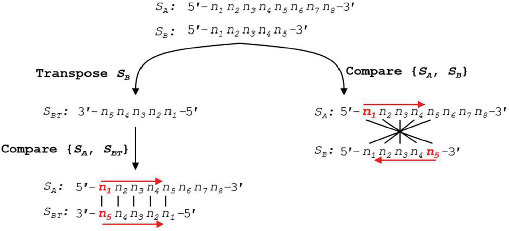
Figure 6 Using a simplified formula to compare two sequences requires the transpose of the second sequence into the 3’–5’ orientation. This transpose costs $\sim$N operations per slip frame, and at worst N$2^{}$ total operation for all slip conditions. A more efficient algorithm can be written without conversion to S${B\mathit{}T}_{}$, where the formula for indexing in S$B_{}$ begins from the end of the sequence, rather than the start. Performance analysis of this reverse indexing algorithm is carried out in Appendix B.3.

We define the variable m as the position within the alignment frame, or the number of nucleobases from the leftmost (5’) base in sequence S$A_{}$. According to Figure 3, the comparison position in S$A_{}$, a$m_{}$, will proceed from the 5’ end, while the comparison index in S$B_{}$, b$m_{}$, will proceed from its 3’ end. The nucleobase indices for comparison in S$A_{}$ and S$B_{}$ (a$m_{}$, b$m_{}$) with slip s$j_{}$ and alignment frame size k$j_{}$ for j $\in$ [1, k${\mathit{range}}_{}$], and an alignment frame index m $\in$ [1, k$j_{}$] can be written for forward slip:

$a_m$	$=m$	(28)
$b_m$	$=L_B-s_j-m+1$	(29)

A similar index pair can be written for backward slip:

$a_m$	$=m+s_j$	(30)
$b_m$	$=L_B-m+1$	(31)

In this way, for all m in a given alignment frame, comparison can be carried out between S$A_{}$(a$m_{}$) and S$B_{}$(b$m_{}$).

A.4 Dimer Indices

This also means that a potential base pair in the given alignment frame can be written as [S$A_{}$(a$m_{}$): S$B_{}$(b$m_{}$)]. For a dimer d of length L$d_{}$ that terminates at frame index m in alignment window k$j_{}$ with slip s$j_{}$, the indices of the base sequence of d in sequences S$A_{}$ and S$B_{}$ (nucleobase sequence indices d$a_{}$ and d$b_{}$, respectively) can be written with the following formulas:

$d_a\in [a_m+1-L_d:a_m]$	(32)
$d_b\in [b_m-1+L_d:b_m]$	(33)

Plugging the definitions of a$m_{}$ (28) and b$m_{}$ (29) for forward slip conditions into (32) and (33), we achieve the following generalized expression for dimer index:

$d_a\in [m+1-L_d:m]$	(34)
$d_b\in [L_B-s_j-m+L_d:L_B-s_j-m+1]$	(35)

The same process can be carried out for backslip conditions, plugging (30) and (31) into (32) and (33):

$d_a\in [m+s_j+1-L_d:m+s_j]$	(36)
$d_b\in [L_B-m+L_d:L_B-m+1]$	(37)

These results are summarized in Tables 5–6 and can be used to directly track and index dimers in a programming environment.

Table 5 Forward slip comparison indices

	Variable		Number
	Name	Definition	in Text
Strand 1 index	$a_m$	$a_m=m$	(28)
Strand 2 index	$b_m$	$b_m=L_B-s_j-m+1$	(29)
Dimer position strand 1	d$a_{}$	$d_a\in [m+1-L_d:m]$	(34)
Dimer position strand 2	d$b_{}$	$d_b\in [L_B-s_j-m+L_d:L_B-s_j-m+1]$	(35)

Table 6 Backward slip comparison indices

	Variable		Number
	Name	Definition	in Text
Strand 1 index	$a_m$	$a_m=m+s_j$	(30)
Strand 2 index	$b_m$	$b_m=L_B-m+1$	(31)
Dimer position strand 1	d$a_{}$	$d_a\in [m+s_j+1-L_d:m+s_j]$	(36)
Dimer position strand 2	d$b_{}$	$d_b\in [L_B-m+L_d:L_B-m+1]$	(37)

Appendix B: Algorithmic Analysis of DNA Heterodimers

In order to design an efficient algorithm for in silico dimer analysis, it is necessary to elucidate the number of operations required to analyze M for heterostructures. A generalized expression can be derived by first looking at a one-node structure, or duplex.

B.1 One-node Structure

Comparison of any set of sequences for dimers requires checking each strand against itself and against each other strand for all allowable slip and alignment conditions. In a single-node network, or DNA duplex, we can see the operations in Figure 7:

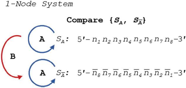
Figure 7 Comparison of S${\mathrm{A}}_{}$ and its complement for heterostructures requires three sets of operations: two self-comparisons (A), and one complement comparison (B).

We can introduce two different types of operations, A and B: Operation A involves the comparison of a single-stranded oligo against itself; whereas Operation B involves the comparison of an oligo and its direct complement, ignoring the case where they are properly aligned, which is precluded by their complementarity. Formulation of these comparisons requires, by definition, that the lengths of the two oligos be identical. The number of comparisons (N) directly scales with the length of the sequences, and involve the summation of the allowable alignment frames, or k${\mathit{size}}_{}$. To do so, we introduce the summorial operator $, which is the additive cousin of the factorial operator:

$x!$	$={\displaystyle \prod _{i=1}^x}i$
$x\$$	$={\displaystyle \prod _{i=1}^x}i$	(38)

The summorial operation can be decomposed into the following formula:

$$x\$=\frac{n(n+1)}{2}$$

(39)

B.1.a Homodimer operation counts (Operation A)

The number of comparisons in A can be calculated by summing all components (k$j_{}$) of forward and backward frames, k${\mathit{size}}_{}$, where the number of slip cases, n${s\mathit{}f}_{}$ and n${s\mathit{}b}_{}$, are equivalent to forward and backward k${r\mathit{}a\mathit{}n\mathit{}g\mathit{}e}_{}$, respectively:

$$N_A=\sum _j^{n_{sf}}{k}_j+\sum _j^{n_{sb}}{k}_j$$

(40)

Substituting (19) for n and (A.2 Frame Alignment) for k$j_{}$ in the left sigma:

${\displaystyle \sum _j^{n_{sf}}}{k}_j$	$={\displaystyle \sum _{j=1}^{L_a}}(L_a-j+1)$
	$=(L_a)\$$
	$={\displaystyle \frac{(L_a)(L_a+1)}{2}}$

Again substituting (20) and (27) in the right sigma:

${\displaystyle \sum _j^{n_{sb}}}{k}_j$	$={\displaystyle \sum _{j=1}^{L_a-1}}(L_a-j)$
	$=(L_a-1)\$$
	$=(L_a)\$-L_a$
	$={\displaystyle \frac{(L_a)(L_a+1)}{2}}-L_a$

Collecting terms, we can simplify to obtain the operation count for A:

$N_A$	$={\displaystyle \frac{(L_a)(L_a+1)}{2}}+{\displaystyle \frac{(L_a)(L_a+1)}{2}}-L_a$
$N_A$	$=L_a^2$	(41)

We can see a practical demonstration of this operation in Figure 8. In this example, sequence S$A_{}$ has a length of 8 nt. Summation of the comparisons across each annealing frame is shown.

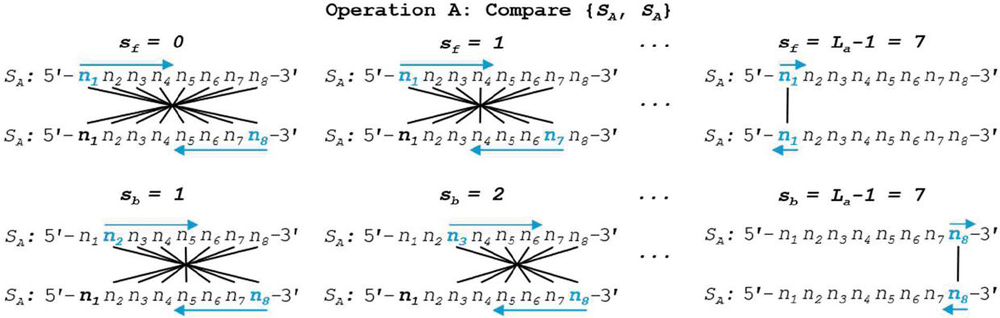
Figure 8 Self-dimerization (Operation A) comparison of generalized single-stranded, 8 nt oligonucleotide S$A_{}$ is shown in both forward and backward slip conditions. Note that, by convention, backslip starts with a value of 1, while forward slip begins at perfect alignment, or a slip value of 0. To speed computation, formulas for the comparison of S$A_{}$ without 5’ and 3’ realignment are shown. This involves the reverse indexing formulas found in Tables 5–6.

Operation A is efficient at order $O(n^2)$ for n nucleotides. In the specific case of Operation A, we can draw lines of symmetry at the halfway point of the alignment frame in the case of even k${\mathit{size}}_{}$, or around the center nucleotide in the case of odd k${\mathit{size}}_{}$, and note that the comparisons will be identical across this line of symmetry (Figure 9). With this in mind, we can reduce the number of comparisons by tracking the even- or oddness of the frame size and performing operations up to, but not past, the line of symmetry. Any dimer that exists once the center of the alignment frame is reached will be doubled in length after omitting odd-length pivot nucleotides. The tracking of frame size modulo 2 requires several floating point operations, and is only practical in high-performance situations for large L. A more efficient Operation A can be seen in Figure 10. This reduced dimerization search operates at roughly $O(\frac{1}{2}{n}^2)$.

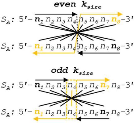
Figure 9 Two different alignment frames are shown for oligonucleotide S$A_{}$, one of even k${\mathit{size}}_{}$ (8 nt) and the other with odd k${\mathit{size}}_{}$ (7 nt). A line of symmetry can be drawn down the middle for the even case, and around the pivot nucleotide for the odd case. Because the nucleotides are identical in the opposing strands, the comparisons across the symmetry lines will also be identical: $(n_1==n_8)=(n_8==n_1)$.

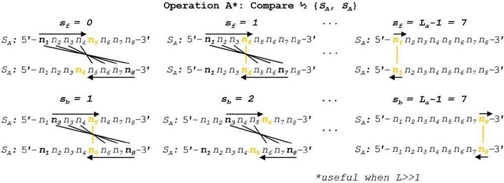
Figure 10 A high-performance algorithm for Operation A is shown, wherein the frame size and evenness are tracked. Comparisons are not continued past the line of symmetry, and any extant dimers that occur at this line are doubled (subtracting 1 nt for odd frame sizes). Note reverse indexing formulas found in Tables 5–6 to account for two 5’–3’ aligned sequences.

B.1.b Heterodimer counting with logical complements (Operation B)

We can sum k${\mathit{size}}_{}$ for Operation B in a similar way, making sure to exclude s$f_{}$ $=$ 0 to avoid counting logical complements as dimers, and we arrive at a general expression. Setting up the problem, we generate an expression identical to (40):

$$N_B=\sum _j^{n_{sf}}{k}_j+\sum _j^{n_{sb}}{k}_j$$

(42)

By disallowing $s_f=0$, we generate identical backslip conditions for both sigmas, which condenses with the application of definitions (20) and (27):

${\displaystyle \sum _j^{n_{sf}}}{k}_j$	$={\displaystyle \sum _j^{n_{sb}}}{k}_j={\displaystyle \sum _{j=1}^{L_a-1}}{L}_a-j$
	$=(L_a-1)\$$
	$={\displaystyle \frac{(L_a-1)(L_a)}{2}}$
$N_B$	$={\displaystyle \frac{(L_a-1)(L_a)}{2}}+{\displaystyle \frac{(L_a-1)(L_a)}{2}}$
$N_B$	$=L_a^2-L_a$	(43)

We can see a practical demonstration of this operation in Figure 11. In this example, sequence S$A_{}$ has a length of 8 nt. Summation of the comparisons across each annealing frame is shown.

Figure 11 Complement dimerization (Operation B) comparison of generalized single-stranded, 8 nt oligonucleotide $S_A$ and its logical complement $S_{\overline{A}}$ is shown in both forward and backward slip conditions.

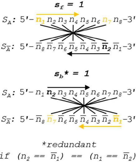
Figure 12 Slip value of 1 is shown for forward and backward slip. We can see that when there is Watson Crick complementarity, these two comparison conditions are identical. A higher performance algorithm in canonical pairing environments can be enacted by omitting backslip, as ($n_2==n_1)=(n_1==n_2)$.

Note that both forward and backward slip start with values of 1 in order to avoid counting complementarity-by-design as a heterodimer. In order to speed computation, formulas for comparison without 5’ and 3’ realignment are shown, which involves the reverse indexing formulas found in Tables 5–6.

Operation B is efficient at order $O(n^2-n)$ for n nucleotides. The number of overall comparisons shown in Figure 11 will include redundant operations when the base pairing rules are symmetric (see Figure 12). This is only true when each nucleobase has one and only one logical complement, which indicates that a full oligonucleotide or dimer substring will have exactly one complement as well. In the case of ion pairing, or any scheme where a nucleobase has multiple complements, the full operation, shown in Figure 8, is necessary. If true DNA Watson Crick rules are in effect, Operation B may be halved in size by omitting backslip, as shown in Figure 13. The updated WC algorithm for Operation B is efficient at order $O(\frac{1}{2}(n^2-n))$.

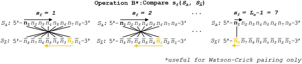
Figure 13 When Watson-Crick or other unitary complement pairing rule system is in effect, backslip may be omitted for symmetry reasons. Tracking the pairing regime does not require significant computation time, and thus tracking the usefulness of this updated algorithm can be considered essential for dimer identification as it will double comparison speed. Reverse indexing formulas for nucleotide position tracking are found in Table 5.

B.1.c Application to a one-node structure (DNA duplex)

For any DNA duplex consisting of two complementary oligonucleotides of equal length (L), we can express the number of comparisons (N) by adding together the operations above. Operation A occurs twice, as each strand must be compared to itself, while Operation B occurs once for the union of the two strands in non-complementary configurations.

$N_{\mathit{duplex}}$	$=2N_A+N_B$
$N_{\mathit{duplex}}$	$=3L^2-L$	(44)

B.2 Multi-node structure

A DNA nanostructure, primer-target complex, or other mixture of oligonucleotide species can be represented as a multi-node network such as the two-node structure shown in Figure 14. As before, the comparisons can be broken down into distinct procedures. Operations A and B return in the same form, and we introduce Operation C, which we define as the alignment and comparison of sequences from disparate nodes. In this operation, we dispense with the requirement that $L_a=L_b$.

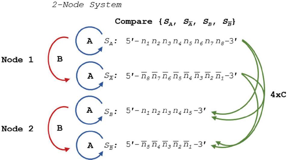
Figure 14 Comparison of nucleotides for dimer search in a two-node structure with three distinct Operations, A, B and C, representing self-comparison, complement comparison, and other sequence comparison, respectively.

B.2.a Heterodimer comparison in disparate nodes (Operation C)

To formulate the number of comparisons, we sum forward and backward k${\mathit{size}}_{}$ vectors with the allowance of s$f_{}$ $=$ 0. Recall that the formulas for k${\mathit{size}}_{}$ are dependent upon the relative lengths of the sequences being compared. As a first assumption, we require that the network be sorted in descending length order, where $L_1\ge L_2\mathrm{\cdots }\ge L_i\ge \mathrm{\cdots }{L}_n$. This requirement comes from the length-dependent derivation of $k_{\mathit{size}}$ (Tables 3, 4). The final form of the formula will be independent of assortment, and we can dispense with this assumption after derivation.

When $L_a\ge L_b$, we can write the following sum, where n${s\mathit{}f}_{}$ and n${s\mathit{}b}_{}$ are the number of slip conditions (k${r\mathit{}a\mathit{}n\mathit{}g\mathit{}e}_{}$) forward and backward, respectively, and k$j_{}$ is the corresponding frame size, similar to (40) and (42):

$$N_C=\sum _j^{n_{sf}}{k}_j+\sum _j^{n_{sb}}{k}_j$$

(45)

The left sigma can be rewritten by again substituting (19) and (A.2 Frame Alignment):

${\displaystyle \sum _j^{n_{sf}}}{k}_j$	$={\displaystyle \sum _{j=1}^{L_b}}(L_b-j+1)$
	$=(L_b)\$$
	$={\displaystyle \frac{(L_b)(L_b+1)}{2}}$	(46)

The righthand sigma can be rewritten by breaking it into two vectors, substituting (20) and (A.2 Frame Alignment). To address the case where L$a_{}$ $\mathrm{=}$ L$b_{}$, it can be noted that (A.2 Frame Alignment) and (27) are equivalent over the region of interest (substitute (20) into (A.2 Frame Alignment) to check):

${\displaystyle \sum _j^{n_{sb}}}{k}_j$	$={\displaystyle \sum _{j=1}^{L_a-L_b}}{L}_b+{\displaystyle \sum _{j=1}^{L_b}}(L_b-j)$
	$=L_b(L_a-L_b)+(L_b-1)\$$	(47)

Collecting terms from (B.2.a Heterodimer comparison in disparate nodes (Operation C)) and (47), we have:

$$N_C=L_b(L_a-L_b+1)+2(L_b-1)\$$$

Simplifying, we arrive at an expression independent of the relative size of L$a_{}$ and L$b_{}$:

$N_C$	$=L_b(L_a-L_b+1)+(L_b-1)(L_b)$
$N_C$	$=L_a{L}_b$	(48)

We can see a practical demonstration of Operation C in Figure 15. In this example, sequence S$A_{}$ has a length of 8 nt, while S$B_{}$ has a length of 5 nt. Note that, by convention, L$A_{}$ $\ge$ L$B_{}$. Operation C is efficient at order of approximately $O(n^2)$ for n nucleotides, or exactly $O(n^2)$ where L$A_{}$ $==$ L$B_{}$. An analysis of the effect of the relative sizes of L$A_{}$ and L$B_{}$ on the order of convergence can be found below in Appendix B.2.d.

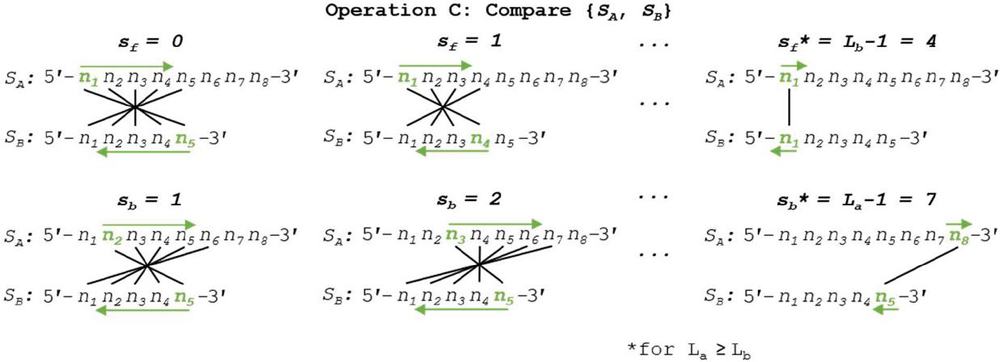
Figure 15 Nucleotide comparison for heterodimer search between disparate oligos (Operation C) is shown. By convention, backward slip starts at a value of 1 to avoid identical comparison, and L$A_{}$ $\ge$ L$B_{}$ to maintain consistency of k${\mathit{size}}_{}$ formulas (Tables 3–4). In practice, this need not be the case, and the relative oligo lengths can be tracked without significant computational overhead.

B.2.b General expression for any network

Returning to Figure 14, we can see that for each node in the system, self-comparison contributes 2A(L$a_{}$)+B(L$b_{}$) operations. Comparison between nodes, for node number D greater than one, we contribute 4C(L$a_{}$,L$b_{}$) comparisons. We can generalize this expression for total comparisons (N) in the following manner:

$N=2{\displaystyle \sum _{i=1}^D}A(i)+{\displaystyle \sum _{i=1}^D}B(i)+4{\displaystyle \sum _{j>i}^D}C(i,j)$

(49)

Substituting in (41), (B.1.b Heterodimer counting with logical complements (Operation B)), and (B.2.a Heterodimer comparison in disparate nodes (Operation C)), we arrive at a general expression for the number of comparisons in any network with D double-stranded nodes:

$N$	$=2{\displaystyle \sum _{i=1}^D}L_i{}^2+{\displaystyle \sum _{i=1}^D}(L_i{}^2-L_i)+4{\displaystyle \sum _i^D}{\displaystyle \sum _{j>i}^D}C(i,j)$
$N$	$={\displaystyle \sum _i^D}(3L_i{}^2-L_i)+4{\displaystyle \sum _{j>i}^D}{L}_i{L}_j$	(50)

B.2.c Comparison of fragmented and single-node networks

An important relationship in computational network analysis is whether the comparison efficiency converges faster in a duplex or a fragmented network. Specifically, will an increased number of nodes for the same number of total base pairs speed or slow computation? To investigate, let us define a network M${\mathrm{1}}_{}$ of D${\mathrm{1}}_{}$ nodes where $D>1$. To perform this analysis, we require that the network M${\mathrm{1}}_{}$ be possessed of nodes with equal lengths, L$n_{}$. We can count the number of operations as before:

$$N_1=\sum _i^{D_1}(3L_i{}^2-L_i)+4\sum _{j>i}^{D_1}{L}_i{L}_j$$

(51)

We can further count the total number of base pairs (B${\mathrm{1}}_{}$) in the network by adding together the lengths of all the nodes (L$i_{}$) in the network:

$$B_1=\sum _i^{D_1}{L}_i$$

(52)

We can then create a M${\mathrm{2}}_{}$ linear structure for comparison containing one node ($D_2=1$) and whose total length (L$q_{}$) is identical to the length of all the nodes in M${\mathrm{1}}_{}$:

$B_2$	$={\displaystyle \sum _1^{D_2}}{L}_i=L_q$	(53)
$B_2$	$=B_1$	(54)

We can then rewrite the number of operations (N${\mathrm{2}}_{}$) in terms of L$q_{}$ and substitute in (52):

$N_2$	$={\displaystyle \sum _i^1}(3L_i{}^2-L_i)$
$N_2$	$=3L_q{}^2-L_q$
$N_2$	$=3{\left({\displaystyle \sum _i^{D_1}}{L}_i\right)}^2-{\displaystyle \sum _i^{D_1}}{L}_i$	(55)

Invoking the requirement that all nodes in M${\mathrm{1}}_{}$ have equal length, $L_n$, we can write:

$$N_2=3D_1^2{L}_n^2-D_1{L}_n$$

(56)

Returning to N${\mathrm{1}}_{}$ we can simplify the number of operations, again requiring that all $L_i=L_j=L_n$. We rewrite (51) using L$n_{}$:

$N_1$	$={\displaystyle \sum _i^{D_1}}(3L_n{}^2-L_n)+4{\displaystyle \sum _i^{D_1}}{\displaystyle \sum _{j>i}^{D_1}}{L}_n^2$
$N_1$	$=D_1(3L_n{}^2-L_n)+4(D_1-1)\$L_n^2$
$N_1$	$=D_1(3L_n{}^2-L_n)+{\displaystyle \frac{4(D_1^2-4D_1)}{2}}{L}_n^2$
$N_1$	$=(2D_1{}^2+D_1)L_n^2+D_1{L}_n$	(57)

We can then take the difference between the two operations (56) and (B.2.c Comparison of fragmented and single-node networks):

$$N_2-N_1=(D^2-D)L_n^2$$

(58)

Normalizing to the sequence length (B${\mathrm{1}}_{}$) of the network, we obtain the following relationship:

${\displaystyle \frac{N_2-N_1}{B_1}}$	$={\displaystyle \frac{(D_1^2-D_1)L_n^2}{D_1{L}_n}}$
${\displaystyle \frac{N_2-N_1}{B}}$	$=D(L_n-1)$	(59)

This formulation suggests that a fragmented network is more efficient to analyze for heterostructures than a one-node network of equal size. This relationship can be seen visualized in Figure 16, where 100 random networks of sizes $D\in [1,30]$ are analyzed, averaged, and compared to (B.2.c Comparison of fragmented and single-node networks) and (58). Ultimately, the speed that is gained by fragmenting a network is lost in the tracking of that geometry, but the trade-off has important implications for algorithm design.

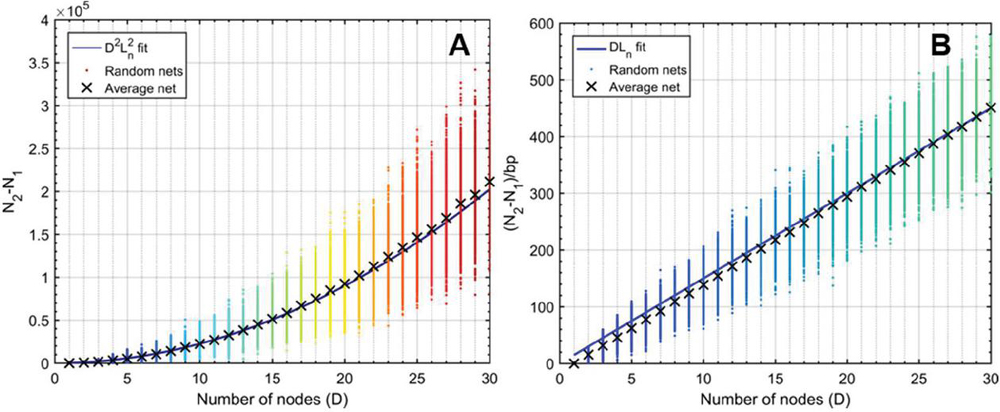
Figure 16 Comparison operation counts in multi-node networks and single-node networks of equal size. Random networks are initialized, analyzed, and averaged for the number of nodes, with 100 trials at each value of D. A) Operation counts for random networks over increasing number of nodes. Overlaying (58) as a fit line for the average behavior serves as a reasonable approximation, where L$n_{}$ is given as the average node size, or L${m\mathit{}a\mathit{}x}_{}$/2, 15 bp. B) Normalizing over the number of base pairs achieves a linear relationship between the difference and the number of nodes. Here, equation (59) serves as a reasonable fit line for the average data at each value of D.

B.2.d Comparison of symmetric and random networks

It is clear that fragmented networks are more efficient to analyze as the number of nodes increases. The analysis thus far has considered symmetric networks where each node has the same length as every other node, a requirement that was imposed to streamline the comparison. How then does the symmetry component affect the computation? We can calculate the difference in operation count between any random network M${\mathrm{0}}_{}$ with total base pairs B${\mathrm{0}}_{}$ and a symmetric network M${\mathrm{1}}_{}$, possessed of the same total length, $B_1=B_0$, and the same number of nodes $D_1=D_0=D$. For network M${\mathrm{1}}_{}$, we know the operation count N${\mathrm{1}}_{}$ in terms of average node L$n_{}$ and D (B.2.c Comparison of fragmented and single-node networks):

$$N_1=(2D^2+D)L_n^2+D{L}_n$$

We have an equation for the operation count N${\mathrm{0}}_{}$ for a generalized network of unspecified node lengths (B.2.b General expression for any network):

$$N_0=\sum _{i=1}^D(3L_i{}^2-L_i)+4\sum _i^D\sum _{j>i}^D{L}_i{L}_j$$

Recall that in a symmetric network, we know the number of base pairs in terms of L$n_{}$ and D:

$$B_1=\sum _1^D{L}_n=D{L}_n$$

(60)

And we know that L$n_{}$ is an average of random node sizes:

$$L_n=\left(\sum _{i=1}^D{L}_i\right)/D$$

(61)

We can then substitute (61) into the definition of N${\mathrm{1}}_{}$ and simplify:

$$N_1=(2D^2+D)\frac{1}{D^2}{\left(\sum _{i=1}^D{L}_i\right)}^2+\left(\sum _{i=1}^D{L}_i\right)$$

(62)

We then subtract N${\mathrm{1}}_{}$ from N${\mathrm{0}}_{}$:

$N_0-N_1=3{\displaystyle \sum _{i=1}^D}L_i{}^2+4{\displaystyle \sum _i^D}{\displaystyle \sum _{j>i}^D}{L}_i{L}_j-\left({\displaystyle \frac{2D^2+D}{D^2}}\right){\left({\displaystyle \sum _{i=1}^D}{L}_i\right)}^2$

(63)

The sums in this sequence must be rearranged to cancel, as ${(\sum x)}^2\ne \sum x^2$. To simplify, we separate the sum squared term into two separate sums:

${\left({\displaystyle \sum _{i=1}^D}{L}_i\right)}^2$	$=\left({\displaystyle \sum _{i=1}^D}{L}_i\right)\left({\displaystyle \sum _{j=1}^D}{L}_j\right)$
	$=\left({\displaystyle \sum _{i=1}^D}{L}_i\right)\left(L_i+{\displaystyle \sum _{j\ne i}^D}{L}_j\right)$
	$={\displaystyle \sum _{i=1}^D}L_i{}^2+{\displaystyle \sum _{i=1}^D}{\displaystyle \sum _{j\ne i}^D}{L}_i{L}_j$

Substituting into (63), we can rearrange:

$N_0-N_1$	$=\left({\displaystyle \frac{D^2-D}{D^2}}\right){\displaystyle \sum _{i=1}^D}L_i{}^2+4{\displaystyle \sum _i^D}{\displaystyle \sum _{j>i}^D}{L}_i{L}_j$
	$\mathrm{\hspace{1em}}-\left({\displaystyle \frac{2D^2+D}{D^2}}\right){\displaystyle \sum _{i=1}^D}{\displaystyle \sum _{j\ne i}^D}{L}_i{L}_j$	(64)

Now we can split the last term into two sums and combine like terms across the expression:

$N_0-N_1$	$=\left({\displaystyle \frac{D^2-D}{D^2}}\right){\displaystyle \sum _{i=1}^D}L_i{}^2+4{\displaystyle \sum _i^D}{\displaystyle \sum _{j>i}^D}{L}_i{L}_j$
	$\mathrm{\hspace{1em}}-\left({\displaystyle \frac{2D^2+D}{D^2}}\right){\displaystyle \sum _{i=1}^D}{\displaystyle \sum _{j<i}^D}{L}_i{L}_j-\left({\displaystyle \frac{2D^2+D}{D^2}}\right){\displaystyle \sum _{i=1}^D}{\displaystyle \sum _{j>i}^D}{L}_i{L}_j$
$N_0-N_1$	$=\left({\displaystyle \frac{D^2-D}{D^2}}\right){\displaystyle \sum _{i=1}^D}L_i{}^2+\left({\displaystyle \frac{2D^2-D}{D^2}}\right){\displaystyle \sum _i^D}{\displaystyle \sum _{j>i}^D}{L}_i{L}_j$
	$\mathrm{\hspace{1em}}+\left({\displaystyle \frac{-2D^2-D}{D^2}}\right){\displaystyle \sum _{i=1}^D}{\displaystyle \sum _{j<i}^D}{L}_i{L}_j$

We then simplify this expression by introducing the constants $\alpha$$m_{}$ and ${\beta }_m$ and splitting into three terms, (65–67):

$N_0-N_1$	$={\displaystyle \sum _{i,j}^D}{\alpha }_m{L}_i{L}_j$	(65)
${\alpha }_m$	$={\displaystyle \frac{{\beta }_m{D}^2-D}{D^2}}$	(66)
${\beta }_m$	$=\{\begin{array}{cc}-2\mathit{\hspace{1em}}\hfill & i<j\hfill \\ 1\mathit{\hspace{1em}}\hfill & i=j\hfill \\ 2\mathit{\hspace{1em}}\hfill & i>j\hfill \end{array}$	(67)

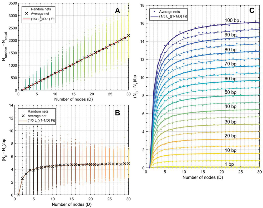
Figure 17 Difference in operation counts between random networks and their symmetric counterparts ($N_0-N_1$). Symmetric networks were obtained by summing averaging the size of all nodes in a given random net, allowing for fractional base pairs. At node numbers $D\in [1,30]$, random lengths were assigned between 1 and 30 bp. At each $D$ value, 100 trials were run. A) The average behavior at each $D$ value for $L_{max}=30bp$ (X marks) was subjected to polynomial fit and determined to correspond to $\frac{1}{3}{L}_n^2(D-1),$ where $L_n$ is $L_{max}/2$, or 15 bp. Data points were obtained using (65) and are identical to data generated without the use of a simplified expression [(50)–(57)]. B) The same experiment was performed and normalized to the total number of base pairs according to (60), where $B={\sum }_i^D{L}_i\sim D{L}_n$. Here the fit line also behaves with $\frac{1}{3}{L}_n(1-\frac{1}{D})$ relationship, which converges to $\frac{1}{3}{L}_n$ for $D\gg 1$. C) Experiments for values of $L_{max}\in [1,100]$ were carried out in the same manner as B. Only the average data are shown with their corresponding fit lines. The value of $L_{max}$ is inset on lines every 10 bp.

If we reassume that all nodes in M${\mathrm{0}}_{}$ are equally sized, we can see that, on average, N${\mathrm{0}}_{}$ is greater than N${\mathrm{1}}_{}$ by approximately L$n_{}$${\mathrm{2}}^{}$, though the meaningfulness of that assertion is questionable. On the whole, (65) will describe the difference in performance between any random network and a symmetric network of equal node number and base pairs. The relationship between random networks and their symmetric counterparts can be seen in Figure 17.

Appendix C: Performance Considerations

In order to speed computation, it is considered best practice to vectorize operations in algorithmic design. In the case of oligonucleotide analysis, this involves avoiding time-intensive character vector comparison. We can see this spelled out in the following two prominent cases.

C.1 Float Conversion

The storage of an oligonucleotide is typically done as a character array, for example: ‘GGACTAG’, where the sequence is read left-to-right to represent the 5’–3’ orientation. Unfortunately, no mathematical operations can be performed on a character array. By contrast, a string converted to a number, either an integer or float data type, can carry out comparisons through subtraction, allowing for a vectorized analysis of sequence composition. Through experimentation (see Appendix C.3 below), double-precision floating point numbers, ‘double’ in Matlab or ‘float’ in Python, demonstrate the shortest nucleotide comparison times. To correspond with one-indexed programming languages like Matlab, [‘ATGC’] can be converted to [1, 2, 3, 4]. In a zero-indexed programming environment, we convert to [0, 1, 2, 3] to promote efficient vectorization. To account for all nucleobase possibilities, we utilize the following convention: [dA, rA $=$ 1.0]; [dT $=$ 2.0]; [dG, rG $=$ 3.0]; [dC, rC $=$ 4.0]; [dC/dG, rC/rG, S $=$ 5.0]; [dA/dT, rA/rT, W $=$ 6.0], [rU $=$ 7.0].

C.2 Comparison by Vector Subtraction

To compare substrings to character elements, a for loop iterates through the array and uses a comparison method such as strcmp(). To identify the complement of a nucleotide substring in a larger oligonucleotide array, we utilize the following comparison matrix for WC and CC pairing conditions:

$$\begin{array}{cc}\hfill \mathrm{WC}\mathit{\hspace{1em}\hspace{1em}\hspace{1em}}\hfill & \hfill \mathrm{CC}\hfill \\ \hfill \begin{array}{c}\hfill {}^{\prime }A^{\prime }\hfill \\ \hfill {}^{\prime }T^{\prime }\hfill \\ \hfill {}^{\prime }G^{\prime }\hfill \\ \hfill {}^{\prime }C^{\prime }\hfill \end{array}:\left[\begin{array}{c}\hfill {}^{\prime }T^{\prime }\hfill \\ \hfill {}^{\prime }A^{\prime }\hfill \\ \hfill {}^{\prime }C^{\prime }\hfill \\ \hfill {}^{\prime }G^{\prime }\hfill \end{array}\right]\mathit{\hspace{1em}\hspace{1em}\hspace{1em}}\hfill & \hfill \begin{array}{c}\hfill {}^{\prime }A^{\prime }\hfill \\ \hfill {}^{\prime }T^{\prime }\hfill \\ \hfill {}^{\prime }G^{\prime }\hfill \\ \hfill {}^{\prime }C^{\prime }\hfill \end{array}:\left[\begin{array}{c}\hfill {}^{\prime }T^{\prime }\hfill \\ \hfill {}^{\prime }A^{\prime }\hfill \\ \hfill {}^{\prime }C^{\prime }\hfill \\ \hfill {}^{\prime }G,C^{\prime }\hfill \end{array}\right]\hfill \end{array}$$

(68)

This comparison algorithm uses two for loops, one to iterate through the oligo array, and the second to iterate through the rule matrix to identify the identity of the base and its possible complements using string comparison. A second string comparison is then carried out to compare complementary characters to the opposing oligonucleotide array. In this way, dimers can be identified within an alignment frame.

A more efficient algorithm stores the oligonucleotide sequence as double-precision floating point number (float64, or double) and subtracts each ‘nucleotide’ from the nth row of float64 rule matrix, where [‘A’,’T’,’G’,’C’] is equivalent to [1,2,3,4]:

$$\begin{array}{cc}\hfill \mathrm{WC}\mathit{\hspace{1em}\hspace{1em}\hspace{1em}}\hfill & \hfill \mathrm{CC}\hfill \\ \hfill \begin{array}{c}\hfill 1\hfill \\ \hfill 2\hfill \\ \hfill 3\hfill \\ \hfill 4\hfill \end{array}:\left[\begin{array}{c}\hfill 2\hfill \\ \hfill 1\hfill \\ \hfill 4\hfill \\ \hfill 3\hfill \end{array}\right]\mathit{\hspace{1em}\hspace{1em}\hspace{1em}}\hfill & \hfill \begin{array}{c}\hfill 1\hfill \\ \hfill 2\hfill \\ \hfill 3\hfill \\ \hfill 4\hfill \end{array}:\left[\begin{array}{c}\hfill 2\hfill \\ \hfill 1\hfill \\ \hfill 4\hfill \\ \hfill 4,3\hfill \end{array}\right]\hfill \end{array}$$

(69)

One loop is used to iterate through the oligonucleotide array. At each base, the row corresponding to the nucleotide identity is subtracted from the complement nucleotide. Where a value of 0 is reached, complementarity is obtained. This eliminates a loop and both expensive character comparisons, speeding computation by two orders of magnitude (see Appendix C.3 below).

In Matlab, this operation utilizes a one-indexed adenine, whereby the first row of the rule matrix in (69) is considered row 1. In a zero-indexed coding environment such as Python, adenine will be converted to 0, and subtraction of row 0 for nucleobase comparison will occur.

C.3 Performance Analysis

Analysis was performed in Matlab to identify the most efficient method of nucleobase comparison. The time to perform a single comparison was averaged across 10$8^{}$ iterations. Comparison of char vector ‘G’ with the second element in ‘TTTATG’ cost an average of 471 ns.

By contrast, subtraction of row 2 from element 2 of the floating point representation of the same sequence took on average 3.65 ns. Though utilizing less disk space, storing the sequence as a single precision floating point number (float32, single) took longer, clocking at 3.89 ns. Finally, even though the rows and columns of a matrix have integer values, storage as an integer (int8, int) took 6.63 ns. These data can be seen in Table 7:

Table 7 Comparison efficiency of various Matlab data structures

Data	Sequence	Complementarity	Average	(xSlower)timeN/
Type	Representation	Rule Matrix	Operation Time	timeDouble
double	[2, 2, 2, 1, 2, 3]	[2, 1, 4, 3]	3.65 ns	–
single	[2, 2, 2, 1, 2, 3]	[2, 1, 4, 3]	3.89 ns	1.06
int	[2, 2, 2, 1, 2, 3]	[2, 1, 4, 3]	6.63 ns	1.81
char	[‘T’,’T’,’T’,’A’,’T’,’G’]	[‘T’, ’A’, ’C’, ’G’]	472 ns	129

There are tens of thousands of nucleotide comparisons to analyze a single DNA nanostructure (B.2.b General expression for any network). Any sequence optimization through iterative algorithms will involve hundreds of millions to billions of comparisons. It is therefore clear that a conversion to double-precision floating point arrays is a critical feature for dimer search, complement generation, and nucleobase identification algorithms, and can enable high-performance optimization of DNA sequences for nanotechnology.

C.4. Reverse Indexing

The tracking of base index inside an alignment frame is an operation requiring relatively few floating point operations. When aligning two sequences to test for complementarity, the usual practice on paper is to take a 5’–3’ oligo and place it adjacent to a 3’–5’ sequence. Though this makes conceptual sense, it requires that the user perform a flip operation on one oligo in an environment where all oligos are stored in the 5’–3’ orientation. In a programming environment, this requires matrix transposition, which uses a relatively large number of floating point operations. An analysis of the time to transpose a floating point ‘oligo’ array of varying length was carried out over 10$6^{}$ iterations, and was determined to cost $\sim$1 $\mu$s per fliplr() operation (Figure 18). A single nanostructure can have thousands of alignment frames; over an iterative time scale, these transpositions will introduce significant delays in sequence design algorithms.

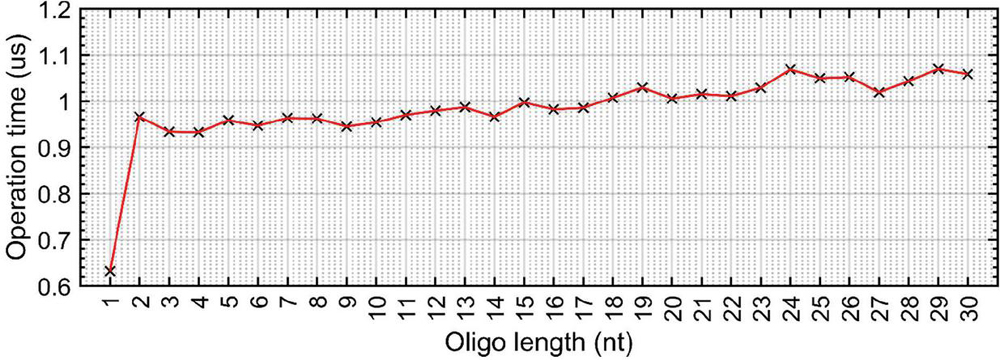
Figure 18 Average time to take a 5’–3’ sequence and use fliplr() to store it in 3’–5’ orientation in a Matlab floating point array. Operation carried out over 10$6^{}$ trials. For all sequence lengths $>$1 nt, transposing the array took approximately 1 $\mu$s. Omitting the first data point, the linear fit equation is approximately: $45ns/nt+920ns$ (R${}^2=0.87$).

To avoid gratuitous transposition of DNA arrays, we introduce reverse indexing, whereby base position in complement strands can be tracked going backwards from the end of the alignment frame. This allows the two oligos of interest to remain in the 5’–3’ orientation. Indexing formulas of this type can be found in (34)–(37) and are summarized in Tables 5–6.

Appendix D: Detailed Algorithm Design and Fitness Evaluation

D.1 UI Component

A nanostructure is a struct() data type with N nodes. Each node is also a data struct() with information about incoming and outgoing edges, sequence, length and a rule matrix which governs allowable mutations. These parameters are entered using a GUI, in which the geometry and sequence of each node is manually specified, as well as its ability to be edited and internal pairing regime. At this stage, certain regions can be restricted to WC or CC parity; while other nodes can be specified as sticky ends by having no complement, no incoming node connections, and uneditable sequences. The user has quite a bit of flexibility over the types of sequences entered and the ways that they connect, allowing for entry of complex nanostructures with heterogeneous local design rules.

D.2 Optimization Criteria Setup

After the user specifies the geometric frame that will be optimized, the model proceeds to the setup stage, in which a parallel pool GA iterator is initialized and run with specific criteria. The runtime environment is initialized with user-defined parameters covering the size and number of solution populations, the size of fitness tournaments and the crossover and mutation rates governing sequence diversity. In addition to standard GA parameters, we introduce environmental variables which will affect the real-time performance and assembly of the nanostructures themselves. Firstly, the user will specify what base pairs are globally available for dimer analysis, akin to specifying the presence or absence of environmental factors such as silver and mercury cations, RNA bases, and orthogonal nucleotides. A global ruleMatrix is established (69), which governs fitness function evaluation across all nodes.

D.3 Iterative Optimization

Populations are built from collections of mutually-interacting solutions that are separated from other populations. The number of total solutions tested is the product of popSize and popNum. The model runs for a set number of iterations, or generations, using the gen number as a stop criterion. To generate a pop, the basic nanostructure frame is subjected to an initial, elevated mutation rate, which causes all editable nodes to be subjected to near-randomization of base pairs allowed in their corresponding ruleMatrix. Setting a low initial mutation rate may be beneficial when continuing to optimize an already-modeled set of sequences. After initializing the data structures and the first generation pop, the model is ready for subsequent iteration. The GA iterator performs the same operations for each cycle: sequence generation, fitness calculation, and pop creation. Owing to the linearly-independent nature of separate solution pools, populations are run in parallel using the parallel computing toolbox in Matlab. Core allocation can be specified at the start of the simulation.

D.3.1 Fitness score calculation

The fitness score is a weighted composite penalty comprised of several criteria, namely: guanine repeats (‘G${\mathrm{N}}_{}$’), GC repeats (‘S${\mathrm{N}}_{}$’), AT repeats (‘W${\mathrm{N}}_{}$’), purine repeats (‘R${\mathrm{N}}_{}$’), pyrimidine repeats (‘Y${\mathrm{n}}_{}$’), nucleobase gaps (‘gap${\mathrm{n}}_{}$’), and heterostructure dimer size (‘D${\mathrm{N}}_{}$’) (see Appendix B). The type of solution will be influenced by the relative weight of these parameters. To allow for user input, the variable dimerWeight is introduced, which corresponds to the stringency of dimer size requirements. This parameter corresponds to the dimer size that is equal in penalty to G$3_{}$, S$4_{}$, R$4_{}$, and Y$4_{}$. In the presence of a gap criterion, a gap size exceeding the user-specified maximum is also weighted similarly with dimers of size dimerWeight (dW). The fitness penalty of the following parameters is identical: D${\mathrm{dW}}_{}$, G$3_{}$, S$4_{}$, W$4_{}$, R$4_{}$, gap$2_{}$. The Y${\mathrm{N}}_{}$ criterion is ignored.

For each solution, histograms of all dimers, guanine repeats, purine repeats, nucleobase gaps, etc. are generated using the indexing and analytical framework established in Section 2 and Appendix B. From these histograms, GC, purine and pyrimidine repeats of size less than 4, guanine repeats and dimers less than size 3, and allowable gaps are all pared from these histograms. The remaining histogram bins are then subjected to a series of exponential functions:

$F$	$={\displaystyle \sum _{i\ge 3}^{n_D}}{c}_{D,i}{10}^{(i-2-dW)}+{\displaystyle \sum _{i\ge 4}^{n_R}}{c}_{R,i}{10}^{(i-2)}+{\displaystyle \sum _{i\ge 4}^{n_W}}{c}_{W,i}{10}^{(i-2)}$
	$\mathrm{\hspace{1em}}+{\displaystyle \sum _{i\ge 4}^{n_S}}{c}_{S,i}{10}^{(i-2)}+{\displaystyle \sum _{i\ge 3}^{n_G}}{c}_{G,i}{10}^{(i-1)}+{\displaystyle \sum _i^{n_{gap}}}{c}_{gap,i}{10}^i$	(70)

In (D.3.1 Fitness score calculation), summation across each histogram bin occurs for repeats of size i, starting at empirically-identified sizes and finishing at the maximum repeat, or n$X_{}$, for each parameter. The number of repeats at each size, $c_i$, corresponds to the histogram bin value at i. This number is multiplied by a decimal exponent containing i and an adjustment value to match the weights of criteria with different critical i values. A solution with better (fewer) repeats will have a smaller fitness value F. As such, the global optimization problem is the minimization of F. Pyrimidine repeats are omitted from the fitness function for redundancy, and GC repeats may be omitted for CC pairing environments to allow polycytosine repeats (this may affect the helical angles and assembly of the constituent nanostructure). Gaps are only included where specified by the user.

Dimer fitness is adjusted by dW or dimerWeight as dimers are of lesser relative importance compared with other types of repeats: a nanostructure may assemble with a size 7 bp heterodimer, while it will not be able to form a B-form duplex with a size 7 nt guanine repeat. The exponential is applied in order to clearly differentiate between the steps in the fitness hill: 5 dimers of size 8 bp are of lesser importance than 2 dimers of size 9 bp. By contrast, 10 dimers of size i will be equal in penalty to 1 dimer of size $\mathit{\text{i}}+1$. In this way, each level of the fitness hill is clearly segregated by repeat size, while the repeat count (c) is weighed in a granular fashion within each step (Figure 19).

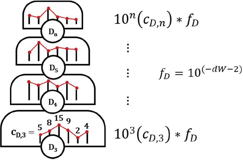
Figure 19 Graphical representation of dimer fitness hill. Each level is of size 10$i^{}$ for a dimer of size i. Within each grade, the number of dimers of each size—the histogram bin count $c_{D,i}$— is the exponent constant. Here, f represents the multiplication factor, or relative weight, of the given fitness characteristic. Different criteria will have different weights, seen in (D.3.1 Fitness score calculation).

The full fitness function can be described in a compact sum, shown in Figure 20. This graphical representation of the different fitness criteria demonstrates the relationship between fitness criteria and their weights. It can be seen that as other criteria pass their minimum penalties, the fitness hill becomes less granular, as the contribution of heterodimers will predominate. Selection of parameter dW by the user will determine the size of heterodimer where this solution characteristic becomes more heavily penalized. A good starting value for dW may be between 8 and 10.

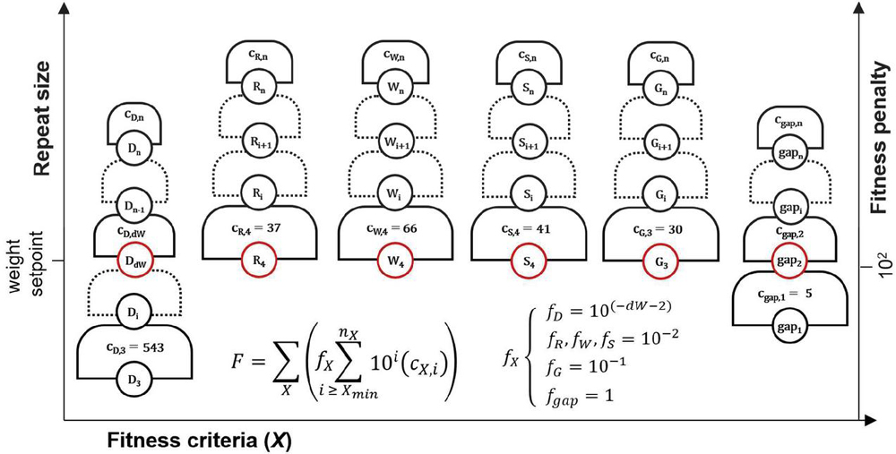
Figure 20 Schematic representation of fitness function (D.3.1 Fitness score calculation). The fitness (F) of a solution is comprised of several sequence design criteria (X): dimers (D), purine repeats (R), AT pair repeats (W), GC pair repeats (S), guanine repeats (G), and nucleobase gaps (gap). Within each criterion, there is a graded fitness hill with levels segregated by the exponential function c*10$i^{}$ for repeat size i and histogram bin count c${X\mathrm{,}i}_{}$. Levels marked in red are weighted equally. The weights are controlled by adjustment factor f$X_{}$. Each repeat type has a maximum recorded value n$X_{}$, and a minimum size X${m\mathit{}i\mathit{}n}_{}$, under which histogram bins are not counted.

The fitness function F for fitness criteria X = [(D)imer, pu(R)ine, (W)eak pair, (S)trong pair, (G)uanine, nucleobase (gap)], repeat size i, repeat count c${X\mathrm{,}i}_{}$, minimum repeat size X${m\mathit{}i\mathit{}n}_{}$, maximum repeat size n$X_{}$, and adjustment factor f may be expressed in compact sum form, as seen in Figure 20:

$F={\displaystyle \sum _X}\left(f_X{\displaystyle \sum _{i\ge X_{min}}^{n_X}}{10}^i(c_{X,i})\right)\mathit{\hspace{1em}}{f}_X\{\begin{array}{c}{f}_D={10}^{(-dW-2)}\hfill \\ f_R,f_W,f_S={10}^{-2}\hfill \\ f_G={10}^{-1}\hfill \\ f_{gap}=1\hfill \end{array}$

(71)

D.3.2 Creating a population for the next generation

Once the fitness scores for a current generation are calculated, these rankings are used to populate the next generation. First, an elitism algorithm is executed in which a specified number of solutions are copied without alteration from the top of the fitness list. If the number of elites meets or exceeds the population size, no optimization will occur. Once elites are copied, a specified number of random solutions are generated where editable nodes are subject to a pseudorandom number generator.

The remaining slots in the next generation pop are filled using tournament style competition. Solutions are selected at random to fill a tournament of specified size, and the fittest individual is chosen. Ties are broken by choosing the first of the solutions selected during tournament filling. A second tournament is carried out, and the two best solutions are subject to a crossover algorithm, in which editable sequence information is exchanged with a specified probability. A random number is rolled $\mathit{\text{r}}=[0,1)$, and if the crossover rate exceeds r, the nucleotides in template and complement strands at that position are swapped using forward and reverse index values. The two modified solutions are then subjected to nucleobase randomization at a specified rate, where editable nucleotides are subjected to a random number roll $\mathit{\text{r}}=[0,1)$. When the mutation rate exceeds the roll, a random base is selected from that node’s ruleMatrix, and if a complement sequence is available, a complementary base is selected at random from the allowable complementary nucleotides in the same row of the ruleMatrix. In this way, two new solutions are generated with information mostly conserved from previous answers based on fitness calculation and tournaments. When there is only one available slot left in the next generation pop, the first new solution to be generated will be selected. Once the population is filled, the generation number is advanced.

D.3.3 Repeat for F2 cross

When the last generation is reached for a given population P$j_{}$, fitness scores are calculated and the best solutions are copied without alteration to a separate population, F${\mathrm{2}}_{}$. The best solutions from all P$j_{}$ are collected and subsequently optimized in the same manner. The F${\mathrm{2}}_{}$ population is subjected to the same runtime parameters as each of the feeder populations. The fittest solution in the final F${\mathrm{2}}_{}$ generation is designated as the end result of the genetic algorithm. This type of forced migration, or gene flow, serves to overcome fitness niches created through the steepness of the fitness landscape by combining disparate solutions.

D.4 Data Analysis and Output

When specified, data analysis across the lifetime of the simulation can be analyzed. In particular, the fitness scores and various metrics can be plotted over iterations and compared with the final F2pop. The parameters displayed are modular and may be chosen with some alteration to plot code. The graphical interface is shown without alteration in Figures 19–21. Figure 21 displays logarithmic fitness data over the lifetime of the simulation. The F2pop (bold) combines the best solutions from the feeder populations and is subject to intense initial competition, followed by slight incremental change over the lifetime of the final simulation. Figures 22–23 show the magnitude and frequency of repetitive segments in the nanostructures, with fitness criteria (X) from (D.3.1 Fitness score calculation)–(71). Repeat sizes are subjected to a weight function to illustrate both the maximum repeat size X$n_{}$ and the abundance of that repeat c${X\mathrm{,}n}_{}$. This function can be expressed as repeat size X$n_{}$ with an additional weight $\mathit{\text{w}}=(0,0.5]$:

$$X_n+0.5(1-e^{c_{X,n}+1}).$$

(72)

Figure 24 shows the nucleobase similarity for all bases and all positions between all members of a nanostructure population. The similarity calculation (S) for nanostructures (M) in a population (P$j_{}$) with total number (L) of nucleotides (b$i_{}$) at position M(i) can be expressed in the following way:

$S={\displaystyle \frac{1}{L}}{\displaystyle \sum _u^N}{\displaystyle \sum _{v>u}^N}{\displaystyle \sum _i^L}g(M_u(i),M_v(i))\mathit{\hspace{1em}}g(b_1,b_2)\{\begin{array}{cc}1\mathit{\hspace{1em}}\hfill & \mathit{if}{b}_1-b_2=0\hfill \\ 0\mathit{\hspace{1em}}\hfill & \mathit{otherwise}\hfill \end{array}$

(73)

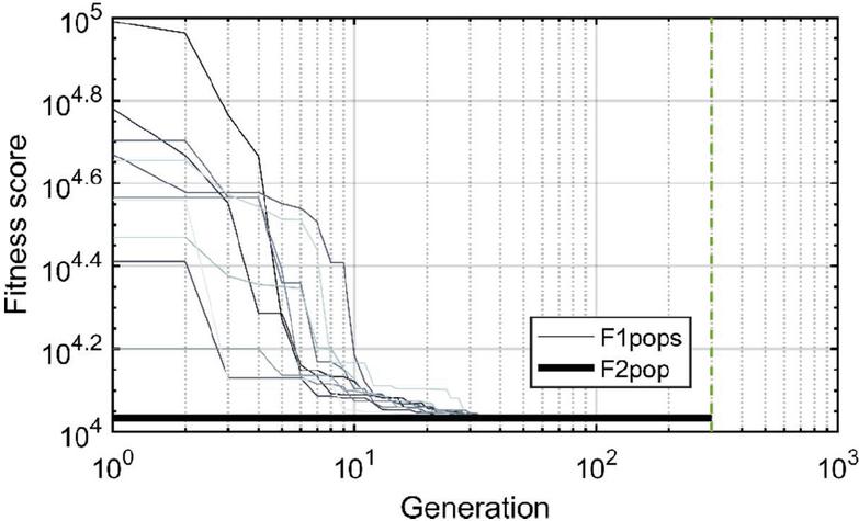
Figure 21 Longitudinal fitness data, plotted on logarithmic axis. The F2pop (marked bold) combines the best solutions of all other populations at the end of their respective simulations. Subsequent optimization selects for the best traits of each of these populations and may arrive at a further-optimized answer.

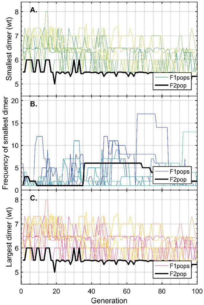
Figure 22 Longitudinal dimer data plotted for F1pops P$j_{}$ (colored lines) and F2pop (bold). A) The largest dimer (D$n_{}$) of the fittest solution in each generation for all pops is shown. In order to show more granular data, the frequency of the dimer c${D\mathrm{,}n}_{}$ is included in this smallest dimer with the weight function (72): $D_n+0.5(1-e^{c_{D,n}+1})$. This function caps the weight of the dimer to $D_n+0.5$. B) The frequency of the largest dimer (c${D\mathrm{,}n}_{}$) from A within a single nanostructure is shown. As a result of the fitness function, dimer count c${D\mathrm{,}i}_{}$ for dimer size D$i_{}$ greater than 10 is counted as equal in weight to a dimer of size D${i\mathrm{+}\mathrm{1}}_{}$, which causes most frequencies to rapidly fall under 10. C) The least fit solution for each generation is plotted in a similar fashion to A. It can be seen from these graphs, which are automatically displayed at the end of simulation, that the F2pop far outperforms the other populations, and that where feeder populations generally reduce the max dimer size D$n_{}$, the F2pop will primarily reduce the histogram bin count c${D\mathrm{,}n}_{}$ for D$n_{}$.

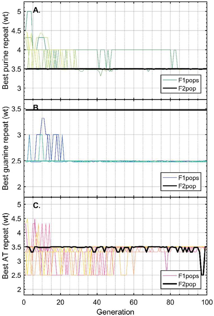
Figure 23 Plots of maximum repeats (X$n_{}$) for varying criteria (X) over all generations for all pops with weight function (72): $X_n+0.5(1-e^{c_{X,n}+1})$. As in Figure 19, the maximum display value for a repeat of size X$n_{}$ is $X_n+0.5$. Criteria shown: A) single-strand purine nucleotide (A,G) repeats (R$n_{}$); B) single-strand guanine nucleotide repeats (G$n_{}$); and C) weak base pair (A:T) repeats (W$n_{}$). Due to the nature of the fitness function, these repeats rapidly drop to the minimum recorded values and experience little change across the lifetime of the simulation.

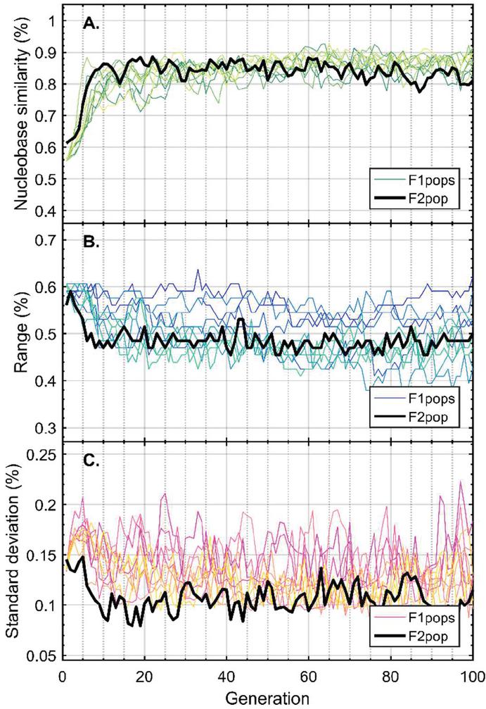
Figure 24 Similarity statistics for all pops over all generations based on (73). A) Average percentage of nucleotides that are identical within nodes across all individual solutions in the population. B) Range between maximum and minimum similarity for all individual solutions in the population at the given generation. C) Standard deviation of similarity scores between all individual solution in the population at the given generation.

Graphical analyses can be utilized to tailor future simulations by analyzing the effects of competition over iterative time scales to select the appropriate runtime parameters.

Appendix E: Runtime Parameter Analysis

When it comes to user experience with the genetic algorithm described here, there are two main metrics that must be considered: fitness of the final best solution, and time of simulation to generate the given solution. The user may adjust the runtime parameters as they see fit in order to reach a high-quality solution in a reasonable amount of time, but it is not always immediately apparent what effect the changes will have. We investigate several parameters and their effects on final solution fitness through statistical analysis of repetitive tests using similar setup states.

E.1 Mutation Rate

A population which is subject to low mutation rate may receive beneficial traits at a rate too slow to be useful to the user, while a population subject to elevated mutation rates may not be able to retain these traits after developing them in the first place. We perform statistical testing of the genetic algorithm for a DAO variant nanostructure (see Section 4), recording fitness and similarity statistics for ten simulations with each runtime setup (Figure 25). Three mutation rates were utilized, 2%, 5% and 10%. Solutions produced by both 2% and 10% mutation rates were both less diverse and less fit than solutions produced in the 5% condition. The fitness of 5% mutation falls at the lower extreme of the error bars for the other conditions, but the solutions are consistently clustered in this higher-fitness region. Results from the 2% and 10% conditions were much more variable in final result, but more internally similar. This suggests the mutation rates that are both too low and too high can lead to fitness niche creation, preventing more optimal solution from being found. It is evident that the computational model should therefore be run with a mutation rate of around 5%.

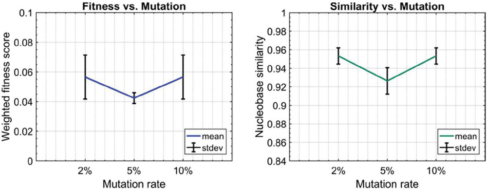
Figure 25 Mutation rate over iterative testing for DAO nanostructure variant at three separate mutation rates: 2%, 5% and 10% (low scores represent better solutions). All other runtime parameters were set to default values. A) F2pop best fitness scores for and accompanying error bars for ten separate instances of running the genetic algorithm. Better solutions for 5% mutation, based on fitness function (71). B) Similarity calculations for the final generation of F2pops based on (73) and accompanying error bars show that a medial mutation rate actually increases population diversity compared with high and low rates.

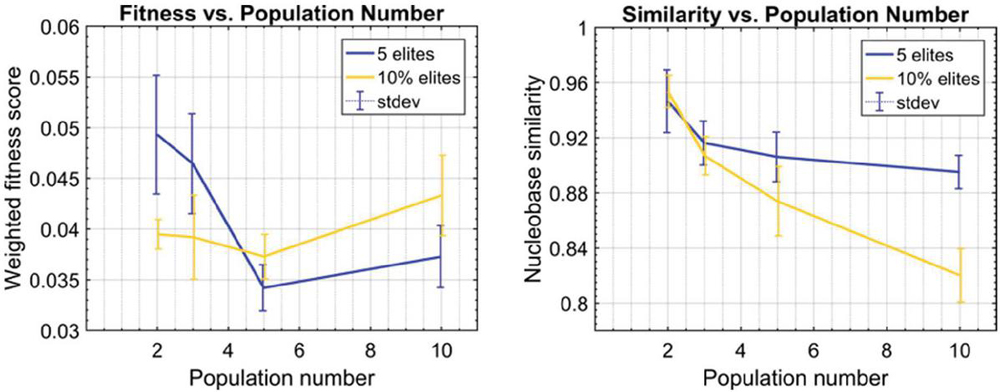
Figure 26 Population size and number with varying rates of elitism for a DAO variant nanostructure. Each data point represents the average of ten independent simulations. Each simulation had 5% mutation and 200 total solutions divided into the number of populations shown on the x-axis. All other runtime parameters were set to default values. To decouple the effects of elitism from population size, the data were collected in two separate cases, one where there were 5 elites in every generation, and again where 10% of the next generation was an unaltered elite. Standard deviation was calculated for each data point ($n=10$). A) Average fitness scores (71) in the best solution for each of the ten independent F2pops. B) Average similarity scores for terminal generation F2pops (73).

E.2 Population Number and Elitism

A similar analysis was performed to extrapolate the relationship between population size and population number (Figure 26). Simulations were performed for 200 solutions, segregated into varying numbers of populations (2,3,5, and 10). By definition, the number of elite solutions in each generation will have an effect independent of actual population size, and in order to decouple the effect of elite fraction in differing population scales, the experiments were repeated with both exactly 5 elites and 10% elites (rounded to integer values). Nanostructures with 10% elitism experienced much less change in fitness for differing population size. By contrast, these populations became much less internally similar as population sizes decreased (increasing population number). Simulations using 5 elite nanostructures experienced greater diversity as population size dropped, but this value became asymptotic as the number of elites occupied 25% of the total population. A sharp increase in overall fitness (more negative fitness score) was exhibited at population numbers greater than three. For both conditions, 5 populations outperformed data collected from 2, 3 or 10 populations, with some question of statistical significance. As a general starting point, the model can be run with 5 populations with 10% elitism for best end fitness and overall solution diversity. Increased simulation times (generation number) may demonstrate better results in these conditions due to diversity retention and relatively smaller fitness niches in these conditions.

References

[1] Mathieu, F. et al. Six-helix bundles designed from DNA. Nano letters 5, 661–665, (2005).

[2] Zheng, J. et al. From molecular to macroscopic via the rational design of a self-assembled 3D DNA crystal. Nature 461, 74, (2009).

[3] Wang, R., Palma, M., Penzo, E. and Wind, S. J. Lithographically directed assembly of one-dimensional DNA nanostructures via bivalent binding interactions. Nano Research 6, 409–417, (2013).

[4] Wang, R., Liu, W. and Seeman, N. C. Prototyping nanorod control: a DNA double helix sheathed within a DNA six-helix bundle. Chemistry & biology 16, 862–867, (2009).

[5] Rich, A. and Davies, D. R. A new two stranded helical structure: polyadenylic acid and polyuridylic acid. Journal of the American Chemical Society 78, 3548–3549, (1956).

[6] Rosenberg, J. M. et al. Double helix at atomic resolution. Nature 243, 150–154, (1973).

[7] Seeman, N. C., Sussman, J. L., Berman, H. M. and Kim, S. Nucleic acid conformation: Crystal structure of a naturally occurring dinucleoside phosphate (UpA). Nature New Biology 233, 90–92, (1971).

[8] Crick, F. and Watson, J. Molecular structure of deoxypentose nucleic acids. Nature 171, 738–740, (1953).

[9] Wang, J. C. Helical repeat of DNA in solution. Proceedings of the National Academy of Sciences 76, 200–203, (1979).

[10] Ono, A. et al. Specific interactions between silver(I) ions and cytosine-cytosine pairs in DNA duplexes. Chem Commun (Camb), 4825–4827, (2008).

[11] Miyake, Y. et al. MercuryII-mediated formation of thymine-HgII-thymine base pairs in DNA duplexes. J Am Chem Soc 128, 2172–2173, (2006).

[12] Wang, A. H. J. et al. Molecular structure of a left-handed double helical DNA fragment at atomic resolution. Nature 282, 680, (1979).

[13] Franklin, R. E. and Gosling, R. G. The structure of sodium thymonucleate fibres. I. The influence of water content. Acta Crystallographica 6, 673–677, (1953).

[14] Leroy, J.-L., Guéron, M., Mergny, J.-L. and Hélène, C. Intramolecular folding of a fragment of the cytosine-rich strand of telomeric DNA into an i-motif. Nucleic acids research 22, 1600–1606, (1994).

[15] Sen, D. and Gilbert, W. Formation of parallel four-stranded complexes by guanine-rich motifs in DNA and its implications for meiosis. Nature 334, 364, (1988).

[16] Seeman, N. C. Nucleic-Acid Junctions and Lattices. Journal of Theoretical Biology 99, 237–247, (1982).

[17] Ding, B., Sha, R. and Seeman, N. C. Pseudohexagonal 2D DNA crystals from double crossover cohesion. Journal of the American Chemical Society 126, 10230–10231, (2004).

[18] Winfree, E., Liu, F. R., Wenzler, L. A. and Seeman, N. C. Design and self-assembly of two-dimensional DNA crystals. Nature 394, 539–544, (1998).

[19] Geary, C., Rothemund, P. W. and Andersen, E. S. RNA nanostructures. A single-stranded architecture for cotranscriptional folding of RNA nanostructures. Science 345, 799–804, (2014).

[20] Rothemund, P. W. Folding DNA to create nanoscale shapes and patterns. Nature 440, 297–302, (2006).

[21] Wang, X. et al. An Organic Semiconductor Organized into 3D DNA Arrays by “Bottom-up” Rational Design. Angewandte Chemie International Edition 56, 6445–6448, (2017).

[22] Mao, C. D., Sun, W. Q. and Seeman, N. C. Designed two-dimensional DNA Holliday junction arrays visualized by atomic force microscopy. Journal of the American Chemical Society 121, 5437–5443, (1999).

[23] Dietz, H., Douglas, S. M. and Shih, W. M. Folding DNA into twisted and curved nanoscale shapes. Science 325, 725–730, (2009).

[24] Zhang, Q. et al. DNA origami as an in vivo drug delivery vehicle for cancer therapy. ACS Nano 8, 6633–6643, (2014).

[25] Pearson, A. C. et al. DNA origami metallized site specifically to form electrically conductive nanowires. J Phys Chem B 116, 10551–10560, (2012).

[26] Zhao, Z., Jacovetty, E. L., Liu, Y. and Yan, H. Encapsulation of gold nanoparticles in a DNA origami cage. Angewandte Chemie International Edition 50, 2041–2044, (2011).

[27] Seeman, N. C. De novo design of sequences for nucleic acid structural engineering. Journal of biomolecular structure and dynamics 8, 573–581, (1990).

[28] Douglas, S. M. et al. Rapid prototyping of 3D DNA-origami shapes with caDNAno. Nucleic acids research 37, 5001–5006, (2009).

[29] Zhu, J., Wei, B., Yuan, Y. and Mi, Y. UNIQUIMER 3D, a software system for structural DNA nanotechnology design, analysis and evaluation. Nucleic acids research 37, 2164–2175, (2009).

[30] Kearse, M. et al. Geneious Basic: an integrated and extendable desktop software platform for the organization and analysis of sequence data. Bioinformatics 28, 1647–1649, (2012).

[31] Oberortner, E., Cheng, J.-F., Hillson, N. J. and Deutsch, S. Streamlining the design-to-build transition with build-optimization software tools. ACS synthetic biology 6, 485–496, (2016).

[32] Zuker, M. Mfold web server for nucleic acid folding and hybridization prediction. Nucleic acids research 31, 3406–3415, (2003).

[33] PrimerQuest${\mathrm{\circledR }}^{}$ program (IDT, Coralville, IA, USA, 2018).

[34] Saiki, R. K. in PCR technology 7–16 (Springer, 1989).

[35] Allawi, H. T. and SantaLucia, J. Thermodynamics and NMR of internal G $\odot$ T mismatches in DNA. Biochemistry 36, 10581–10594, (1997).

[36] Peyret, N., Seneviratne, P. A., Allawi, H. T. and SantaLucia, J., Jr. Nearest-neighbor thermodynamics and NMR of DNA sequences with internal A.A, C.C, G.G, and T.T mismatches. Biochemistry 38, 3468–3477, (1999).

[37] Kaur, H., Arora, A., Wengel, J. and Maiti, S. Thermodynamic, Counterion, and Hydration Effects for the Incorporation of Locked Nucleic Acid Nucleotides into DNA Duplexes. Biochemistry 45, 7347–7355, (2006).

[38] Xia, T. et al. Thermodynamic Parameters for an Expanded Nearest-Neighbor Model for Formation of RNA Duplexes with Watson-Crick Base Pairs. Biochemistry 37, 14719–14735, (1998).

[39] Nakano, S.-i., Fujimoto, M., Hara, H. and Sugimoto, N. Nucleic acid duplex stability: influence of base composition on cation effects. Nucleic acids research 27, 2957–2965, (1999).

[40] Owczarzy, R., Moreira, B. G., You, Y., Behlke, M. A. and Walder, J. A. Predicting stability of DNA duplexes in solutions containing magnesium and monovalent cations. Biochemistry 47, 5336–5353, (2008).

[41] Vecchioni, S., Capece, M. C., Toomey, E., Rothschild, L. and Wind, S. J. Methods of Synthesis and Characterization of Conductive DNA Nanowires Based on Metal Ion-Mediated Base Pairing for Single-Molecule Electronics. Journal of Self-Assembly and Molecular Electronics (SAME) 6, 61–90, (2018).

[42] Dairaku, T. et al. Structure Determination of an AgI-Mediated Cytosine–Cytosine Base Pair within DNA Duplex in Solution with 1H/15N/109Ag NMR Spectroscopy. Chemistry-A European Journal 22, 13028–13031, (2016).

[43] Torigoe, H. et al. Thermodynamic and structural properties of the specific binding between Ag(+) ion and C:C mismatched base pair in duplex DNA to form C-Ag-C metal-mediated base pair. Biochimie 94, 2431–2440, (2012).

[44] Holland, J. H. Adaptation in natural and artificial systems: an introductory analysis with applications to biology, control, and artificial intelligence. (MIT press, 1992).

[45] Konak, A., Coit, D. W. and Smith, A. E. Multi-objective optimization using genetic algorithms: A tutorial. Reliability Engineering & System Safety 91, 992–1007, (2006).

[46] Wu, J.-S., Lee, C., Wu, C.-C. and Shiue, Y.-L. Primer design using genetic algorithm. Bioinformatics 20, 1710–1717, (2004).

[47] Rinker, S., Ke, Y., Liu, Y., Chhabra, R. and Yan, H. Self-assembled DNA nanostructures for distance-dependent multivalent ligand–protein binding. Nature nanotechnology 3, 418, (2008).

[48] Liu, D., Park, S. H., Reif, J. H. and LaBean, T. H. DNA nanotubes self-assembled from triple-crossover tiles as templates for conductive nanowires. Proceedings of the National Academy of Sciences 101, 717–722, (2004).

[49] Seeman, N. C. DNA nicks and nodes and nanotechnology. Nano letters 1, 22–26, (2001).

[50] Fardian-Melamed, N. et al. Electronic Level Structure of Silver-Intercalated Cytosine Nanowires. Nano Letters, (2020).

[51] Livshits, G. I. et al. Long-range charge transport in single G-quadruplex DNA molecules. Nature nanotechnology 9, 1040–1046, (2014).

[52] Hush, N. and Cheung, A. S. Ionization potentials and donor properties of nucleic acid bases and related compounds. Chemical Physics Letters 34, 11–13, (1975).

Journal of Self-Assembly and Molecular Electronics, Vol. 1, 17–76.
doi: 10.13052/jsame2245-8824.2022.002
This is an Open Access publication. © 2023 the Author(s). All rights reserved.