Modeling Charge Transport and Dynamics in Biomolecular Systems
Received 3 December 2012; Accepted 10 December 2012
Journal of Self-Assembly and Molecular Electronics, Vol. 1, 1–39.
doi: 10.13052/same2245-4551.111
Copyright © 2013 River Publishers. All rights reserved.
R. Gutierrez1, G. Cuniberti1, 2
- 1Institute for Materials Science and Max Bergmann Center of Biomaterials, Dresden University of Technology, 01062 Dresden, Germany
- 2Division of IT Convergence Engineering and National Center for Nanomaterials Technology, POSTECH, Pohang 790-784, Republic of Korea; e-mail: projects@nano.tu-dresden.de
Abstract
Charge transport at the molecular scale builds the cornerstone of molecular electronics (ME), a novel paradigm aiming at the realization of nanoscale electronics via tailored molecular functionalities. Biomolecular electronics, lying at the borderline between physics, chemistry and biology, can be considered as a sub-field of ME. In particular, the potential applications of DNA oligomers either as template or as active device element in ME have strongly drawn the attention of both experimentalist and theoreticians in the past years. While exploiting the self-assembling and self-recognition properties of DNA based molecular systems is meanwhile a well-established field, the potential of such biomolecules as active devices is much less clear mainly due to the poorly understood charge conduction mechanisms. One key component in any theoretical description of charge migration in biomolecular systems, and hence in DNA oligomers, is the inclusion of conformational fluctuations and their coupling to the transport process. The treatment of such a problem affords to consider dynamical effects in a non-perturbative way in contrast to, e.g., conventional bulk materials. Here we present an overview of recent work aiming at combining molecular dynamic simulations and electronic structure calculations with charge transport in coarse-grained effective model Hamiltonians. This hybrid methodology provides a common theoretical starting point to treat charge transfer/transport in strongly structurally fluctuating molecular-scale physical systems.
Keywords
- Electronic structure
- biomolecules
- molecular dynamics
- quantum transport
1. Introduction
Can a DNA molecular wire mediate charge transport, i.e., support an electrical current? This question has attracted a considerable attention in the past 20 years, mainly triggered by two facts: first, the emergence of molecular electronics [1–4], which opened the perspective of realizing electronic functions at the molecular level and thus of exploiting DNA self-assembling and self-recognition properties [5–7]; second, by the demonstration of long-range hole transfer in different DNA oligomers in solution in the groups of Barton [8–13], Giese [14, 15], Lewis [16], Schuster [17–19], and Michel-Beyerle [14,20]. These experiments revealed electron transfer occurring over distances as long as 200 Å, which was in so far surprising, as the highly disordered structure of natural DNA – related to a quasi-random base pair sequence – should lead to a considerable degree of charge localization. Mechanisms based on thermally activated incoherent hole hopping have been successful in describing hole transfer in solution [20, 28–30].
However, when coming to investigate experimentally charge transport properties, i.e. the electrical response of DNA when contacted by metallic electrodes, the situation became considerably less clear. Indeed, a variety of partially contradictory experimental results has been obtained in the past years for double-strand (ds) DNA oligomers [19, 21–27]. This situation hints not only at the difficulties encountered to carry out well-controlled transport measurements, but also at the strong sensitivity of charge migration to several factors, including (i) the specific base sequence of the probed molecules, (ii) the structure of DNA (whether in A or B form) which can lead to a quantitative difference in the overlap of the π-electrons of the stacked bases, (iii) the length of the sequences – longer chains may be deformed due to structural instability – so that any kinks and defects in the DNA structure introduced in this way may distort the DNA π-system, and (iv) the DNA-metal contact topology and electronic structure.
Meanwhile, some experiments [25, 26, 39] have shown in a reliable way that charge transport can take place through single short DNA segments. Xu et al. [25] and Cohen et al. [26] addressed dsDNA while Liu et al. [39] focused on G4. Concerning the dsDNA, both experiments found currents of 100–150 nA at about 1 V. In [25], electrical transport through covalently Au-contacted double-stranded DNA in aqueous solution was measured, where the native form of the DNA is preserved. The I –V curves show a rather smooth ohmic profile with considerably large currents up to 150 nA at 0.8 V. The experimental approach of Cohen et al. [26] was based on measuring current through suspended dsDNA molecules connected between a metal substrate and a gold nanoparticle contacted to an AFM conducting tip. Currents of the order of 220 nA at 2.0 V were measured. Interestingly, the length and base sequence of DNA in these two experiments were completely different. Unfortunately, systematic investigations (within a given experimental setup) on base sequence, length, and the temperature dependence of charge transport are still missing, so that the theoretical analysis of possible charge transport pathways faces big challenges [40]. Initial modeling of charge transport was mainly based on effective Hamiltonians with fixed electronic parameters and describing e.g hole transport through the highest occupied molecular orbitals (HOMO) of the bases [41–47] (see also [48, 49] for recent reviews). Model Hamiltonians clearly offer the possibility to explore different charge transport scenarios in a relatively flexible way, but they also contain usually many parameters which are difficult to estimate. This limits the predictive power of those models in case of complex biomolecular systems. On the other hand, first-principle calculations [50–63] performed on static structures can provide accurate values for the electronic couplings but can hardly deal with the full transport problem. As a result, the development of methodologies exploiting the advantages of both approaches become highly desirable.
An important factor governing charge transfer/transport is the biomolecular structural dynamics: several important studies in the chemical physics community have highlighted the crucial role played by dynamical fluctuations in favoring or hindering hole migration [30–38, 61, 64–72]. Hence, we may expect that transport of charges when DNA is contacted by electrodes can only be understood in the context of a dynamical approach which includes the coupling of the electronic system to conformational degrees of freedom, resulting in fully or partially incoherent charge propagation. Indeed, strong conformational dynamics and a related spectrum of different time scales seem to be ubiquitous for biomolecules, as shown e.g., in the modulation of the kinetics of electron transfer during the early stages of the photosynthetic reaction cycle [73], by the analysis of dispersed kinetics [74, 75], or by fluorescense correlation spectroscopy [76]. The treatment of dynamical effects in DNA transport calculations has been, however, addressed only recently either in the frame of pure model Hamiltonians [47, 77–80] or by including information from first principle calculations and molecular dynamics (MD) simulations [67, 69, 81–84].
A realistic inclusion of the influence of dynamical effects onto the transport properties can however only be achieved in our view via hybrid methodologies combining a reliable description of the biomolecular dynamics and electronic structure with quantum transport calculations. The present paper will introduce such a methodology which has been recently developed [81–83, 85–88]. This approach allows to consider the influence of structural fluctuations and solvent effects onto the electronic structure of DNA oligomers. Hereby we use a density-functional (DFT) based fragment-orbital method, which provides a very efficient way to compute the charge transfer parameters along nanosecond molecular dynamic trajectories. Solvation effects are described using a hybrid quantum mechanics/molecular mechanics (QM/MM) coupling scheme. The combination of the method with coarse-grained Hamiltonian models opens the way to study charge transport in complex systems where the interaction with dynamical degrees of freedom plays a fundamental role.
The paper is organized as follows. In the next section we present a model Hamiltonian approach including coupling to specific vibrational degrees of freedom that was used to describe charge transport through standing DNA sequences [26]. The goal of the section is twofold: first to introduce Green function techniques and to show how to treat analytically such problems; second to illustrate what are the intrinsic limitations of approaches based only on model Hamiltonians. In Section 3 we shall then to introduce the computational methodology combining classical molecular dynamic simulations with DFT based electronic structure calculations along the MD trajectory. An efficient coarse-graining is hereby achieved by using fragment orbitals. The resulting effective electronic structure can be mapped onto a linear tight-binding chain with time-dependent electronic parameters. Charge transport can be then investigated along two different but complementary ways: by computing quantum mechanical transmission probabilities along the MD trajectory and performing time averages (Section 3.2) or by mapping the time dependent electronic Hamiltonian onto a model describing the interaction of a static (time averaged) electronic system with a dissipative bosonic environment (Section 4). The main advantage of this second approach is the possibility to describe charge transport beyond the coherent limit. More importantly, the quantities characterizing the bath (spectral density) can be fully determined in terms of time correlation functions of the electronic parameters.
2. Model Hamiltonian Approaches to Charge Transport in DNA Molecular Wires: Standing DNA Oligomers
In the context of charge transport, model Hamiltonian formulations have been extensively applied to address the role played by different physical parameters in determining the efficiency of charge migration through different DNA oligomers. Cuniberti et al. [48] offer a recent overview of different classes of such tight-binding based models commonly used in the past years to compute the charge transport characteristics of DNA wires.
In this section we will present an example on how a model Hamiltonian approach can be used to describe some experimental findings. We pursue hereby two main goals: (i) to show how analytical methods based on Green functions can be applied to deal with the coupling to vibrational excitations in a typical minimal model, and (ii) to demonstrate what is the main drawback of a model treatment of transport, namely, the appearance of a number of free parameters, which are in general difficult to obtain from first-principle calculations. This second aspect is crucial since the complexity of DNA molecules makes a full ab initio estimation of such parameters very challenging and the possible transport scenarios do dramatically depend on the specific values these parameters can take.
The reference point for the theoretical treatment were single molecule experiments performed at the group of D. Porath [26]. In brief, a thiolated 26 bases long single-stranded DNA (ssDNA) with a non-homogeneous sequence was adsorbed on a gold surface to create a dense monolayer. The ssDNA molecules had a thiol-modified linker end group (CH2)3-SH at the 3’-end (see Figure 1(a)). The monolayer was then exposed to a solution of the complimentary ssDNA bound to gold nanoparticles (GNP) via a thiol linker. Upon incubation of ssDNA-GNP conjugates on ssDNA- functionalized gold surface, a certain density of dsDNA attached at one end to the gold surface and at the other end to GNP was formed. A metal coated AFM tip was used to form an electrical contact to protruding GNP and perform electrical measurements across dsDNA. Figure 1(b) shows an AFM image of several GNPs, indicating the position of the hybridized dsDNA on the background of the ssDNA monolayer. The recorded current voltage curves, shown in Figure 1(c) demonstrate in a clear and reproducible way, the ability of ∼9 nm long dsDNA to conduct relatively high currents (> 200 nA), when the molecule is not attached to a hard surface along its backbone and when charge can be injected efficiently through a chemical bond. Such behavior was measured for many dsDNA molecules on tens of samples and with various tips and humidity conditions with similar results.
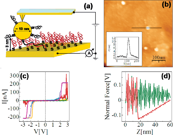
Figure 1 (a) Scheme of the experimental setup showing dithiolated dsDNA chemically bonded to two metal electrodes (upper – GNP, lower – gold surface). The base sequence is given by 5’-CAT TAA TGC TAT GCA GAA AAT CTT AG-3’-(CH2)3-SH. (b) AFM topography image showing a top view of the sample. The GNPs mark the position of the hybridized dsDNA. (c) Collection of I–V curves from different samples. (d) An F–Z curve of one of the curves in (c), (green – forward, red – backward) demonstrating the tip-GNP adhesion (red line) without pressing the GNP through the monolayer. Reprinted with permission from [79]. © 2006 American Physical Society (DOI: 10.1103/PhysRevB.74.235105).
From a theoretical point of view, the central aim is to formulate a minimal model describing the DNA electronic structure and the coupling to the electrodes (metallic surface and GNP modified AFM tip) [79]. For this, we adopt the perspective that to describe low-energy quantum transport within a single-particle picture, only the frontier π orbitals of the base pairs are relevant. The starting point will be then a planar ladder model with a single orbital per lattice site within a nearest-neighbor tight-binding picture as shown Figure 2. Ladder models have been previously used by different authors to study quantum transport in DNA duplexes [43, 46, 89–92]. The Hamilton operator describing the ladder and its coupling to left (L) and right (R) electronic reservoirs is given by

Figure 2 Upper panel: Schematic representation of the double-strand DNA with the experimentally relevant base-pair sequence [26]. The (CH2)3-SH linker groups are omitted for simplicity (see the text for details). Lower panel: Two-strand ladder used to mimic the double-strand structure of a DNA molecule. L and R refer to left and right electrodes, respectively. The coupling terms to the electrodes Γℓ,α,ℓ = X, , α = L, R are assumed to be energy-independent constants. Reprinted with permission from [79]. © 2006 American Physical Society (DOI: 10.1103/PhysRevB.74.235105).
In the above expression, X, refer to the two strands of the ladder, ∊r,ℓ are energies at site ℓ on strand r, tr,ℓ,ℓ+1 are the corresponding nearest-neighbor electronic hopping integrals along the two strands while t⊥,ℓ describes the inter-strand hopping. To have an estimation of the onsite energies, values obtained by Mehrez and Anantram [60] using density-functional theory (DFT) were taken. Considering electron transport, we chose ∊G = 1.14 eV, ∊C = −1.06 eV, ∊A = 0.26 eV, ∊T = −0.93 eV. More difficult is the choice of the intra- and inter-strand electronic transfer integrals. They will be more sensitive to the specific base sequence considered. For the sake of simplicity and in order to reduce the number of model parameters a simple parameterization is adopted taking homogeneous hopping along both strands, i.e. tr,ℓ,ℓ+1 = tX = t = t ∼ 0.25–0.27 eV and t⊥,ℓ = tX ∼ 0.2–0.3 eV. We remark that the hopping integrals are considered as effective parameters, thus keeping some freedom in the choice of their specific values. Electronic correlations [46] or structural fluctuations mediated by the coupling to other vibrational degrees of freedom (see the next paragraphs) can lead to a strong renormalization of the bare electronic coupling. The interaction with the electronic reservoirs will be described in the most simple way by invoking the wide-band approximation, i.e. neglecting the energy dependence of the lead self-energies (see below).
To model the coupling to vibrational degrees of freedom we consider the case of long-wave length optical modes with constant frequencies Ωα, e.g., long wave-length torsional modes and assume they couple to the total charge density operator of the ladder. This approximation can be justified for long-wave length distortions. In other words, the strength of the electron-vibron interaction λ is assumed to be site-independent. The total Hamiltonian thus reads [79]:
To deal with the transport problem using this Hamiltonian model we will use Green function techniques which offer a powerful methodology to cover different transport regimes as well as to treat the coupling between different degrees of freedom. In a first step, a Lang–Firsov (LF) unitary transformation [93] is performed in order to remove the electron-vibron interaction. The LF-generator is given by , which is basically a shift operator for the harmonic oscillator position. The parameter gα = λα/Ωα gives an effective measure of the electron-vibron coupling strength. As a result of the LF transformation, the onsite energies ∊r,ℓ are shifted to with being the so called polaron shift. Renormalization effects in the tunneling Hamiltonian will be neglected in the following.
For the transport problem, the standard current expression for lead p=L,R as derived by Meir and Wingreen [94] can be used:
and then the LF unitary transformation is performed under the trace going over to transformed Green functions. In the previous equation, are the lead spectral functions, is the Fermi function of the p-lead and are the corresponding electrochemical potentials. Within the wide-band limit in the electrode coupling, the following 2N ×2N ladder-lead energy-independent coupling matrices can be defined:
Now define the fermionic vector operator (see Figure 2 for reference):
Lesser- and greater-matrix Green functions (GF) can then be introduced as
Since Eq. (3) does not explicitly contain information on the specific structure of the “molecular” Hamiltonian, we can now transform the lesser- and greater-GF as well as the lead spectral functions to the polaron representation. The operator Ψ transforms according to , where . Thus, we obtain and similar for . Performing an approximate decoupling in this expression into polaronic and vibronic components one obtains:
with a similar expression holding for the lesser-than GF by changing the time argument t by −t in Φ(t).
For a single vibrational mode, the vibron correlation function Φ(t) can be exactly evaluated [93]:
where and g = λ/Ω. It follows then for the Fourier transformed lesser and greater GFs:
where +(−) corresponds to < (>). The bare lesser- and greater-GF can now be obtained from the kinetic equation , since the full electron-vibron coupling is already contained in the prefactor function φn(τ ). The leads self-energy matrices are given in the wide-band limit by i and , respectively. Using these expressions, the total symmetrized current in the stationary state IT = (IL − IR)/2 is given by [79]
where is the conventional expression for the transmission coefficient in terms of the molecular Green function G(E), which satisfies the Dyson-equation: . The above result for the current has a clear physical interpretation. So, e.g., a term like describes an electron in the left lead which tunnels into the molecular region, emits n vibrons of frequency Ω and tunnels out into the right lead. However, it can only go into empty states, hence the Pauli blocking factor . Other terms can be interpreted along the same lines, when one additionally substitutes electrons by holes.
Finally, a spectral density A(E, V ) can be defined as
Figure 3(a) shows the electronic band structure of an infinite periodic array of the 26-base-pairs DNA molecule without considering charge-vibron interactions. The strongly fragmented energy spectrum is a result of the small hopping integrals and the inhomogeneous onsite energy distribution. We may thus rather speak of valence and conduction manifolds as of true dense electronic bands [56]. In Figure 3(a) we also show schematically the positions of the conduction and valence manifolds of a periodic poly(GC) reference system (open rectangles). Figures 3(b)–(d) show the spectral density at zero voltage of the finite DNA ladder contacted by electrodes in three different ways: (b) only the 3’-ends, (c) only the 5’-ends, and (d) all four ends of the double-strand are contacted. Though the general effect consists in broadening of the electronic manifolds, we also see that depending on the way the molecule is contacted to the leads the electronic states will be affected in different ways. Thus, e.g., states around 1.7 eV above the Fermi level are considerably more broadened than states closer to EF.
Considering now the coupling to vibrational degrees of freedom in the ladder, one should notice that the probability of opening inelastic transport channels by emission or absorption of n vibrons becomes higher with increasing thermal energy kBT and/or electron-vibron coupling g. As a result, the spectral density A(E) will consist of a series of elastic peaks (corresponding to n = 0) plus vibron satellites (n ≠ 0).
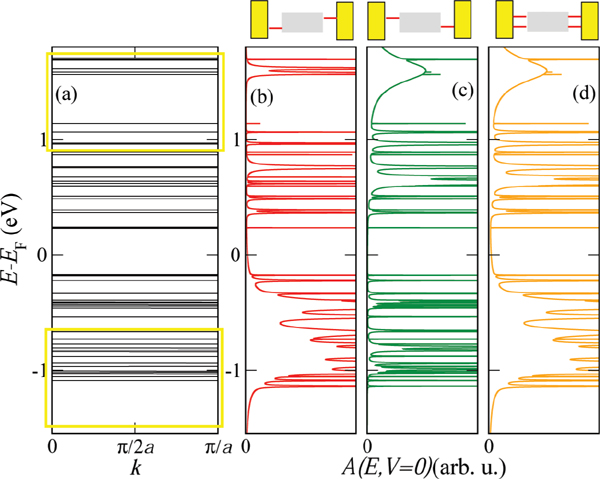
Figure 3 (a) Tight-binding electronic band structure of an infinite DNA system, obtained by a periodic repetition of the 26-base sequence of Cohen et al. [26]. The open yellow rectangles indicate for reference the approximate position of the bands for a periodic poly(GC) oligomer. (b)–(d) Spectral density A(E, V = 0), which at zero voltage coincides with the projected density of states onto the molecular region, for the finite size DNA chain contacted in different ways by left and right electrodes (see Figure 2). Reprinted with permission from [79]. © 2006 American Physical Society (DOI: 10.1103/PhysRevB.74.235105).
Figure 4 shows the influence of the coupling to the vibron mode on the magnitude of the current and of the zero-current gap. The slope of the I – V curves is considerably reduced with increasing g. The corresponding spectral densities at V ∼ 1.5 V (see Figure 4, lower panel) show broadening due to the emergence of an increasing number of vibron satellites (inelastic channels) with larger coupling, but at the same time a redistribution of spectral weights takes place. This is simply the result of a sum rule . The reason for the current reduction can be qualitatively understood by looking at the spectral density. The reduction in the intensity of A(E) will clearly lead to a reduction in the current at a fixed voltage, since it is basically the area under A(E, V = const.) within the energy window [EF − eV /2,EF + eV /2] which really matters. Notice also the increase of the zero-current gap with increasing electron-vibron coupling (vibron blockade), which is related to the exponential suppression of transitions between low-energy vibronic states [95]. Alternatively, this can be interpreted as an increase of the effective mass of the polaron which thus leads to its localization and to a blocking of transport at low energies.

Figure 4 Dependence of the current on the effective electron-vibron coupling strength g = λ/Ω at room temperature. With increasing coupling the total current is reduced and the zero-current gap is enhanced. The lower panels show the spectral density at a fixed bias voltage V ∼ 1.5 V for different values of g. Reprinted with permission from [79]. © 2006 American Physical Society (DOI: 10.1103/PhysRevB.74.235105).
The measured I –V characteristics [26] can be described semi-quantitatively by reformulating the previous model to include two vibrational excitations. The extension of the model is straightforward and details can be found in [79]. Figure 5 shows two experimental curves and the corresponding theoretical I –V plots. The values used for the charge-vibron coupling (λ1 = 15(35) meV, λ2 = 15(20) meV) and vibron frequencies (Ω1 = 20 meV, Ω2 = 6 meV) for the yellow (black) theoretical curves have reasonable orders of magnitude for low-frequency modes, see e.g. [96].
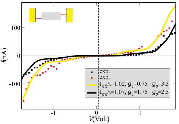
Figure 5 Theoretical curves (solid lines) compared with two different I –V curves as obtained on suspended double-strand DNA oligomers contacted by a GNP [26]. In both cases the temperature and the coupling to the electrodes were kept fixed at T = 300 K and , respectively. Reprinted with permission from [79]. © 2006 American Physical Society (DOI: 10.1103/PhysRevB.74.235105).
The theoretical approach presented in this section highlights the advantages of a model based formulation: (i) low computational cost, (ii) the possibility of obtaining analytical results to analyze limiting cases, and (iii) to cover different physical regimes, like e.g., strong or weak coupling to vibrational modes. However, also the main drawback of a pure model Hamiltonian approach to transport in complex systems can be clearly appreciated: the results can strongly depend on the parameter choice, the number of parameters usually growing with the increase in complexity of the models. Since a purely ab initio based description of transport in complex biomolecular systems is not feasible, it is thus desirable to develop methodologies able to bridge the gap between reliable electronic structure calculations and transport models. The next section will be devoted to present such an approach.
3. Structural Fluctuations in Biomolecular Systems: Bridging Molecular Dynamics with Transport Models
In this section, a methodology [81–83, 85–88] is described which uses a hybrid approach based on a combination of molecular dynamics simulations and electronic structure calculations with a mapping of the time-fluctuating electronic structure along the MD trajectory onto coarse-grained transport models. The key issue is that in this way the number of free parameters in the model formulation is reduced to a large extent. Moreover, the degree of coarse-graining by the formulation of the charge transport model can be progressively improved in a controlled way by adding stepwise information drawn from the electronic structure calculations. In the following the transport problem will be approached from two complementary points of view. In the first one charge transport will be addressed via the computation of time averaged transmission functions, i.e., at regular snapshots ti along the MD trajectory the electronic structure is calculated and from there a quantum mechanical transmission T(E,ti) is computed, thus generating a time dependent T(E,ti) which is then averaged over the simulation time. In the second approach, a model is formulated which describes the coupling of the electronic system to a bosonic bath which comprises internal vibrations and solvent effects. The bath encodes the dynamical information drawn from the MD simulations. The bath spectral density can then be calculated from time series generated during the MD run.
3.1. Electronic Structure and Fragment Orbital Approach
We will first describe the strategy used to calculate in a very efficient way the electronic structure of an arbitrary DNA sequence (the method can be of course applied to other biomolecular systems or to organic stacks) [81–83, 85–88]. The immediate goal is to map the electronic structure onto a tight-binding model with time-dependent electronic coupling and onsite energies. The tight-binding Hamiltonian takes the form
The onsite energies ∊i and the nearest-neighbor hopping integrals Vij characterize, respectively, effective ionization energies and electronic couplings of the molecular fragments (see below). The evaluation of these parameters is done by using the SCC-DFTB method [97] combined with a fragment orbital

Figure 6 Left panel: Schematic representation of the fragment orbital method used to perform a coarse-graining of the DNA electronic structure. A fragment consists of a single base pair (not including the sugar phosphate backbones). As explained in the text, the hopping matrix elements Vj,j+1 between nearest-neighbor fragments are computed using the molecular orbital basis of the isolated base pairs. These calculations are then carried out at snapshots along the molecular dynamics trajectory hence leading to time dependent electronic structure parameters. By keeping only one relevant orbital per fragment, the electronic structure can be mapped onto that of a linear chain (right panel). Reprinted with permission from [83]. © 2010, Institute of Physics.
and
The molecular orbitals φi and φj are, e.g., the highest-occupied molecular orbitals (HOMO) of the DNA bases i and j. Depending on the definition of the FOs, different tight-binding models may be designed. In our case, we use a minimal approach where the DNA electronic structure will be mapped onto a linear chain. The FOs are obtained by performing SCC-DFTB calculations of the isolated fragments, i.e., the individual nucleotide pairs in this case.
Performing an LCAO expansion
the coupling and overlap integrals in the molecular-orbital (MO) basis can be evaluated as
and
Hμν and Sμν are the Hamilton and overlap matrices in the atomic basis set as evaluated with the SCC-DFTB method [87].
The effect of environment, i.e. the electrostatic field of the DNA backbone, the water molecules and the counter-ions, is taken into account through the following QM/MM Hamiltonian:
qδ are Mulliken charges in the QM region and QA are charges in the MM region, i.e. the DNA backbone, counter-ions and water molecules. The coupling to the environment is therefore explicitly described via the interactions with the QA charges. In the following, the calculation scheme based on the complete expression in Eq. (17) will be denoted as QM/MM, while neglecting the last term will be denoted as “vacuo”. The matrix Vij is built from non-orthogonal orbitals φi and φj , so that it will renormalized appropriately [87, 88].
3.2. Time-Averaged Transmission Function and Charge Transport through Linear Chains
To formulate a transport Hamiltonian, the coupling to left (L) and right (R) electrodes needs to be included. In a standard way, a tunnel Hamiltonian is used which will be treated later on within the wide band limit (see Section 2). The full Hamiltonian reads as follows [82]:
Within the Landauer approach, the transmission function at a given instant of time ti along the MD trajectory T(E,ti) for the previous model can be written as
where γL and γR are effective coupling terms to the L and R electrodes within the wide-band approximation, respectively. G1N (E, ti) is the 1,N-matrix element of the chain Green’s function, which can be calculated via a matrix Dyson equation:
Notice that the above expressions refer to transport characteristics at a given time ti along the MD trajectory. Thus, a time series of transmission functions will be generated which is then averaged over the simulation time.
3.3. Molecular Dynamics Methodology
There are a variety of different standard software to perform classical MD simulations of biological systems. In the approach described here, the AMBER-parm99 force field [99] with the parmBSC0 extension [100] as implemented in the GROMACS [101] software package was employed.
After a standard heating procedure followed by a 1 ns of equilibration phase which is discarded afterwards, a 30 ns MD run with a time step of 2 fs was used. The simulations were carried out in a rectangular box with periodic boundary conditions and filled with 5500 TIP3P [102] water molecules and 20 sodium counterions for neutralization. Snapshots of the molecular structures were saved every 1 ps, for which the charge transfer parameters were calculated with the SCC-DFTB-FO approach as described above. To assess the effect of environment, these parameters were computed with and without the external charges in Eq. (17).
3.4. Charge Transport and Dynamics in Short DNA Sequences
Figure 7(a) shows the calculated transmission for various ideal (static) BDNA sequences. As expected, the transmission spectrum consists of a set of resonances which can be related to the eigenvalues of the corresponding Hamiltonian matrices. Due to the very small values of the electronic coupling parameters, these resonances lie very close to the onsite energies of the respective fragments. Also expected are the reduced values of the transmission for inhomogeneous sequences due to the increased energy gaps arising from the differences in the ionization potentials from base to base.
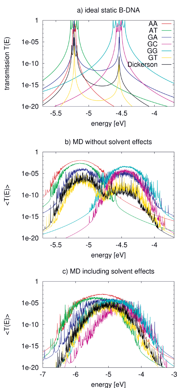
Figure 7 Transmission of the ideal chain (a) including dynamical effects (b) and the effect of environment (c) for various DNA sequences. Note the broader energy range in (c). Reprinted with permission from [82]. © 2009 American Institute of Physics.
Table 1 Electronic couplings Vij for hole transfer in idealized static A and B-DNA without QM/MM environemnt compared to MD averaged values with standard deviations including the QM/MM environment, for helical parameters of the idealized A and B-DNA, see [103] and [104], all values in eV. Reprinted with permission from [82]. © 2009 American Institute of Physics.
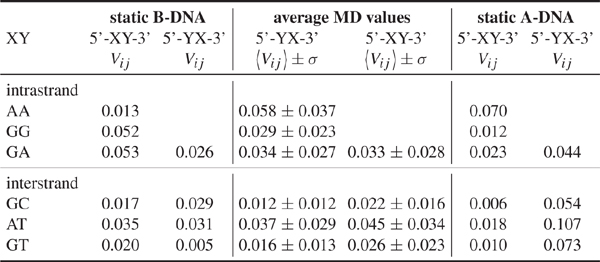
In a second step the coupling parameters are now evaluated along the MD trajectories but omitting the QM/MM term (QA) in Eq. (17). Table 1 shows the MD-averaged couplings in comparison to those of the ideal A- and B-DNA structures. Notice the differences in the coupling when comparing with the static conformations. This results strongly suggests the averaged MD structures being significantly different from the ideal ones [88]. The role of fluctuations is further reflected in the variances σ which are of the same order of magnitude as the averages themselves. These results are nearly independent of the interaction with solvent, indicating that the electronic coupling fluctuations are mainly dominated by the mutual orientation of the base pairs and are not sensitive to the electrostatic coupling to the environment [88].
Figure 7(b) shows the transmission for the various sequences including only the internal dynamics. As a result of the broad distribution of the onsite energies, the transmission spectrum broadens. Further, the dynamical disorder of onsite energies increases the transmission of low-conducting (static) structures, while it decreases it for the “high-conducting” ones. This can be understood by taking into account that the fluctuations of the onsite energies lead to conformations for the “mixed” sequences, such as poly(GA), poly(GT), and the Dickerson dodecamer, where the effective energy gaps become smaller than in the idealized static structures. Therefore, CT-active conformations arise due to the dynamics. On the contrary, the homogeneous sequences become effectively disordered due to the dynamical fluctuations thus reducing the transmission.
To include the effect of DNA backbone, water and counter-ions, the Hamiltonian in Eq. (17) is used to calculate the new electronic coupling and onsite energy parameters. The electric field induced by the water molecules leads to large fluctuations of the onsite energies in the order of 0.4 eV compared to only 0.14 eV without the environment. Also the averages, are shifted by 0.2–0.3 eV to lower energies. Figure 7(c) shows the transmission of the DNA species in the presence of electrostatic field induced by the environment. Since the environment does not affect the electronic coupling strongly, the main difference from Figure 7(b) arises from the larger fluctuations of onsite energy values. As a result of the wider distribution of onsite energies as well as the environment-induced energy shifts, the transmission spectra become considerably broader.
Two interesting points can also be seen in Figure 7(c). First, poly(A) shows the largest transmission, in contrast to the static case where poly(G) is better conducting. Second, the transmission of the heterogeneous species like poly(GA), poly(GT) and the Dickerson dodecamer sequence increases substantially compared to the idealized, static case, indicating that the fluctuations of onsite energies may lead to conformations with smaller effective onsite-disorder.
3.5. Correlations Matter
Several theoretical studies of DNA conduction have used static disorder to address the influence of the solvent or of inhomogeneous base sequences [42, 43, 45]. However, the question arises whether temporal (dynamical) correlations are important in determining the charge transfer efficiency. Taking as a en example the case of a poly(A) heptamer, this issue has been analyzed in some detail. To progressively increase the degree of correlations, three different cases for the probability distribution of the site energies have been chosen: (i) the Anderson model [105], where the onsite energies are randomly drawn from a square-box distribution of width w with uniform probability . The box width is , where σ(∊) is the standard deviation of onsite energies resulting from the MD simulations (σ ∼ 0.4eV); (ii) a PDF model where the onsite energies are drawn randomly from a normal distribution P(∊i) at each site i of the chain, but with no inter-site correlations. These distributions were however obtained from MD simulations; (iii) the full time series are used encoding all relevant time correlations.
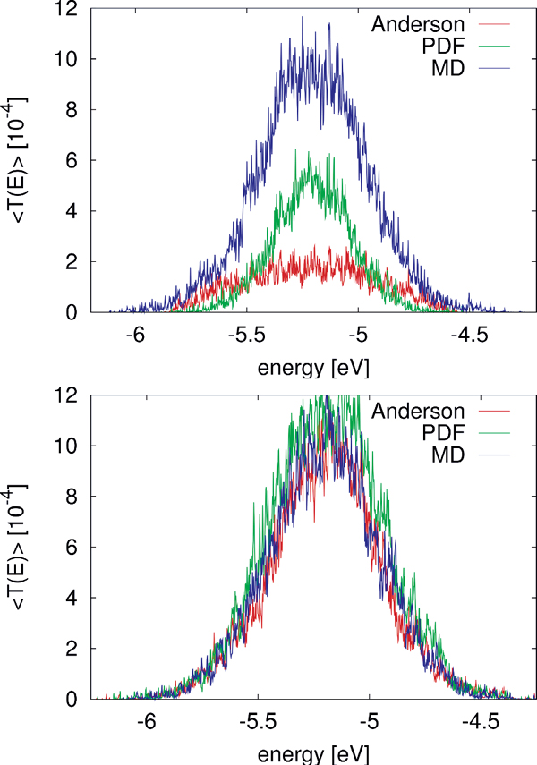
Figure 8 Comparison of for the MD simulation of a poly(A) heptamer with two statistical models. Top panel: The average transmission function is calculated for onsite energies from the MD simulations time series (blue); for onsite energies drawn from the respective probability distribution functions on each site (green); and the Anderson model (red) where all onsite energies are randomly drawn from a square-box distribution. Bottom panel: the original MD time series of onsite energies is used, the same for the three models, while  is calculated for electronic couplings Vij from the original MD time series (blue); for Vij drawn from their respective probability distribution functions (green); and the Anderson model (red), respectively. Reprinted with permission from [82]. © 2009 American Institute of Physics.
To make the results comparable, the electronic couplings are taken constant Vij = 0.05 eV. The average transmission of the poly(A) heptamer for the three cases is shown in the top panel of Figure 8. Clearly, the Anderson model largely suppresses transport (low average transmission) hinting at the potential relevance of correlated fluctuations. Neglecting non-local correlations as in the PDF model but still using a more realistic distribution function of the site energies leads to an increase of the transmission probability. The maximal transmission is obtained when including the full time series in the calculation, which is a clear indicator that non-local (site-to-site) correlations are crucial in determining the charge transport efficiency. Notice that the influence of correlations in the hopping integrals does not seem to be as dramatic as for the onsite energies (bottom panel of Figure 8).
3.6. Conformational Analysis
To analyze in more detail the role played by the conformational dynamical disorder, two effective measures can be introduced [82]:
The standard deviation ∑ is calculated for the ∊i along the chain and has an evident meaning. Large values of ∑ indicate large differences of neighboring site-energies. Note, the index N in and means that averaging is performed for the N sites along the chain. The other parameter Π is motivated by the form of Greens function matrix element G1N (E) required to calculate the transmission function, which scales approximately as the product of electronic couplings in the weak coupling case, i.e. when the ratio , where V and Δ∊ are typical hopping matrix elements and energy gap parameters, respectively. Thus, this quantity determines the transmission efficiency of the system; small values of Π account for conformations with small couplings along the DNA chain. In order to reduce the complexity of further analysis we additionally define the value Tmax as simply the maximum of a given transmission function T(E). Note, that the value Tmax can be located anywhere within the respective energy range. All three parameters ∑, Π and Tmax are now calculated for 30,000 snapshots along the 30 ns MD trajectory of a poly(G) heptamer.
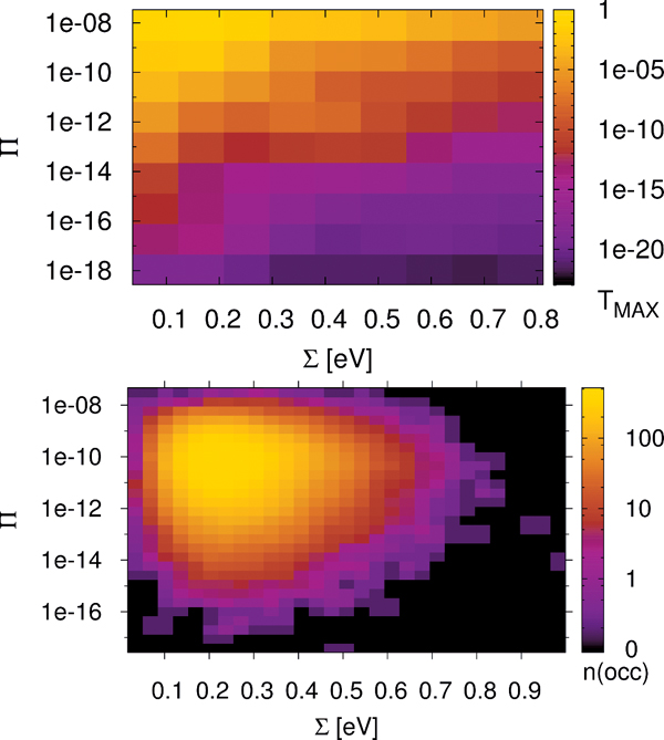
Figure 9 Statistical analysis of Tmax in a poly(G) heptamer, for the 30 ns data with electronic parameters for every ps (30,000 DNA conformations). Tmax depending on ∑ and Π (top); number of conformations found in a given interval of ∑ and Π (bottom). Reprinted with permission from [82]. © 2009 Amer ican Institute of Physics.
The results are shown in Figure 9 (top panel). We see that none of the measures ∑ and Π alone is able to describe the conformations of high conduction, but both seem to contribute nearly linearly to the transmission (note the logarithmic scales for Π and Tmax). However, for the transport active conformations, small ∑ and large Π values are required.
Figure 9 (top panel) also shows that TMAX depends more strongly on Π than on ∑. For instance, if Π is kept fixed at 10−8, then the maximum transmission TMAX is still at least 10−7 for all values of ∑. On the other hand, keeping the parameter ∑ fixed makes Tmax decrease to almost 10−17 even for the smallest value of ∑. The bottom panel of Figure 9 shows the corresponding occupation plot. Here, it is quantified how many conformations exhibit a certain combination of ∑ and Π parameters. It seems that the number of transport active conformations with appropriate electronic couplings and onsite energies is very small. Most conformations have ∑ values of about 10Π10 and ∑ values of about 0.25 eV, and are therefore “CT-silent”. This analysis is obviously subjected to the restriction that transport characteristics have been calculated using (time averaged) transmission functions, which eventually cannot catch the full transport pathways of the system (decoherence effects are clearly not included here). Nevertheless, this approach is able to shed light onto the concept of CT active or silent conformations.
4. Charge Transport in Dissipative Environments
In the previous section charge transport was treated within Landauer theory and the influence of dynamical fluctuations was effectively included via a time average procedure. Here, we will change the perspective and go back to model Hamiltonian formulations where the coupling to dynamical degrees of freedom is explicitly included. However, with the methodology presented in the preceding section we will now be in the position to parametrize not only the electronic structure part of the model but also the interaction with the vibrational system. As a representative example, we focus on the Dickerson dodecamer with the sequence 3′−GCGCTTAACGGC−5′ and for which the effect of the dynamical fluctuations becomes very clear (see Section 3, especially Figure 7). As introduced before, the starting point is a time-dependent electronic Hamiltonian for a linear chain where both onsite energies ∊j(t) and electronic coupling terms are drawn from the MD simulations:
Since Eq. (23) contains random variables through the time series. We are, strictly speaking, confronted with the problem of dealing with charge transport in an stochastic Hamiltonian. This is a complex task which has been addressed, e.g., in the context of exciton transport [106–109], but also to some degree in electron transfer theories [110–112]. Here, we adopt a different point of view and reformulate this model in a way that the coupling to dynamical degrees of freedom is split off and included in a bosonic bath, which can thus be explicitly treated. The Hamiltonian can be rewritten in the following way [83]:
where
The time averages (over the corresponding time series) of the electronic parameters and have been split off to provide a zero-order electronic Hamiltonian which contains dynamical effects on a mean-field-like level. The effect of the fluctuations around these averages is hidden in the vibrational bath, which is assumed to be a collection of a large (N → ∞) number of harmonic oscillators in thermal equilibrium at temperature kBT. The bath will be characterized by a spectral density J(ω) which can also be extracted from the MD simulations. The model is completed by including the interaction with electrodes along the same lines as in Eqs. (1) and (19).
The previous model relies on some basic assumptions that can be substantiated by the results of the MD simulations: (i) The complex DNA dynamics can be well mimic within the harmonic approximation by using a continuous vibrational spectrum; (ii) the simulations show that local onsite energy fluctuations are much stronger in presence of a solvent than those of the electronic hopping integrals, so that we assume that the bath is coupled only diagonally to the charge density fluctuations; and (iii) fluctuations on different sites display rather similar statistical properties, so that the charge-bath coupling λα is taken to be independent of the site j. A typical correlation function of the onsite energy fluctuations is displayed in Figure 10 for the Dickerson dodecamer in both solvent and vacuum (no electrostatic environment) conditions as well as one case of off-diagonal correlations between nearest-neighbor site energies (inset). Also shown are fits to stretched exponentials, which are in general a compact way of representing a fit to a sum of single exponential functions, i.e. the presence of different time scales in the problem, leading to long time tails in the correlation functions. As extensively discussed in, e.g., [113], the emergence of long-time tails can be generally understood in terms of the ratio between typical charge propagation times and typical time scales for the dynamical fluctuations of the system. Especially, long fluctuation time scales (compared with typical charge propagation times) can induce deviations from a purely single exponential behavior. From the figure it becomes clear that off-diagonal correlations decay on shorter time scales as the local ones, so that on a first approximation to neglect them can be justified (although in general they can not be fully excluded); further, the decay of the correlations for the vacuum simulations is considerably much faster than in a solvent indicating the strong influence of the latter in gating the electronic structure of the biomolecule.
Similar to Section 2, we perform a polaron transformation of the Hamiltonian Eq. (24), using the generator
The parameter gives an effective measure of the electron-vibron coupling strength. As a result, we obtain a Hamiltonian with decoupled electronic and vibronic parts and where the onsite energies are shifted as
The retarded Green function of the system is now an entangled electronic-vibronic object that can not be treated exactly; we thus decouple it in the approximate way, see also Eq. (6) [79, 114]:

Figure 10 Normalized auto-correlation function and averaged nearest-neighbor correlation function (inset) of the onsite energy fluctuations. The solid lines are fits to stretched exponentials. Reprinted with permission from [83]. © 2010 Institute of Physics.
In this equation, ) is the Heaviside function and the pure bosonic operator . In the last row of Eq. (25) we can pass to the continuum limit and express φ(t) in terms of the bath spectral density J(ω) [115]:
Using standard techniques [83, 94], we can then write an expression for the electrical current:
Here, the transmission-like function T(E) is given by and is calculated without including the coupling to the bosonic bath, which is already taken into account by the Φ(E) functions.
4.1. Getting the Bath Spectral Density from Molecular Dynamics
A central issue in the reformulation of the transport problem is how to get the bath spectral density J(ω) from the information encoded in the time series of the electronic parameters. We will explain this point by using a much simpler toy model consisting of a single time dependent level whose site energy is a Gaussian random variable:
Using equation of motion techniques for the Green function of the system we arrive at the following solution (within the wide band approximation in the coupling to the electrodes:
Where . Averaging the Green function over the distribution of the random variable δ (t) and performing a cumulant expansion up to second order (Gaussian distribution) yields now in the energy-space:
which is the formally exact solution of the problem if the correlation function is specified. We may now look at the same problem from a different point of view by considering the coupling of a single site with time-independent onsite energy to a continuum of vibrational excitations. Along similar lines as in the previous section, we can write the retarded Green function as
where φ(t) has been already defined in Eq. (26). By comparison of Eqs.( 30) and (31), it becomes clear that there should exist a relation between the (real) correlation function and the real part of φ(t). Writing Re φ(t) as
we can conclude that
Upon inversion, we get
which provides the desired relation between the bath spectral properties and the correlation function of the onsite energy fluctuations.
4.2. Charge Transport in the Dickerson Dodecamer
We have applied this formulation to study charge transport through the Dickerson dodecamer in presence and absence of solvent effects. To first illustrate the influence of the solvent, in Figure 11 the time averaged onsite energies along the chain are displayed. Remarkably, the presence of the solvent “smoothes” the averaged energy profile (though the amplitude of the fluctuations clearly becomes stronger).
In Figure 12 the current calculated with Eq. (27) is shown for the two cases of interest. Due to the presence of tunnel barriers in the wire which, on average, are not fully compensated by the gating effect of the environment, the absolute current values are rather small when compared with those of homogeneous sequences (not shown) [81]. However, the current including the solvent is roughly fifteen times larger than for that obtained from the simulations in vacuum. Although our model Hamiltonian in Eq. (25) does not fully contain all the dynamical correlations encoded in the time dependent electronic parameters, we nevertheless expect that their inclusion would lead to an even further increase of the difference between solvent and vacuum results. This nicely demonstrates that coupling to dynamical degrees of freedom is crucial when dealing with charge migration in soft systems and that the basic effects can still be catch by effective model Hamiltonians whenever appropriate (realistic) parameterizations are carried out. The possibility to parameterize the bath spectral density J(ω) using the information obtained from the MD time series makes our approach very efficient. We remark that the scheme presented here is obviously not limited to the treatment of DNA but it can equally well be applied to deal with charge migration in other complex systems like molecular organic crystals or polymers, where charge dynamics and coupling to fluctuating environments plays an important role [110–112, 116–120].
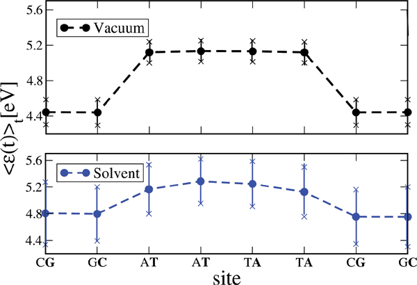
Figure 11 Time average of the absolute value of the onsite energies of the Dickerson dodecamer for simulations in vacuum (upper panel) and in solvent (lower panel). Notice that the averaged energy profile in presence of the solvent becomes smoother but also the fluctuations around the averages are stronger. This smoothing reduces the energy barriers between the sites and hence favors charge migration. Reprinted with permission from [83]. © 2010 Institute of Physics.
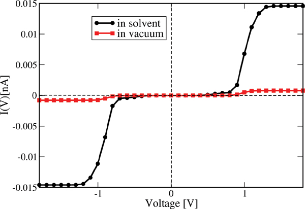
Figure 12 Electrical current for the Dickerson dodecamer in both vacuum (no solvent) and including the solvent. The current is considerably enhanced upon inclusion of solvent fluctuations, nicely demonstrating the strong gating effect of the latter onto the energy profile of the DNA chain. Reprinted with permission from [83]. © 2010 Institute of Physics.
5. Conclusions
In contrast to hole transfer in solution, where there seems to be common agreement about the microscopic charge migration mechanism (incoherent hopping processes), the clarification of the most relevant charge transport pathways in short DNA oligomers still remains elusive. This may be due to the fact, on one side, that well-controlled electrical transport experiments are difficult to perform with biomolecules, so that general trends and dependencies on base sequences, temperature, etc. have not been fully elucidated. On the other side, the intrinsic complexity of biomolecules make a description in terms of simple models very challenging and as a consequence, many results can be questionable if the physically relevant parameter region is not well defined. The fundamental role played by the structural dynamics and the need to include such effects in a non-perturbative way in charge transport calculations further increases the problems faced by theoreticians when dealing with the biomolecular electrical response. In this paper, we have focused on recently developed methodologies which try to address all these previously mentioned problems by combining molecular dynamics simulations with electronic structure calculations to parameterize effective model Hamiltonians able to deal with different transport scenarios in DNA oligomers. The main advantage of this approach is the possibility to develop a controlled coarse-graining of the electronic structure, which in its turn allows tuning the degree of complexity of the model Hamiltonians for transport. Additionally, the methodology is flexible enough to be transferred to the study of charge transport and dynamics in other systems like polymers or organic crystals, thus providing a common platform to treat with such issues. Obviously, several points remain still open and should be addressed in the future. We only mention two of them: How reliable is a quantum mechanically computed electronic structure along a classical molecular dynamic trajectory, i.e., with geometries obtained using classical interaction potentials? How strong is the influence of a charge injected into the system onto the underlying electronic structure? This latter effect is usually neglected in transport calculations, but it has been recently shown that it has an influence in the prediction of, e.g., the onset of diffusive transport in organic stacks [121], so that we may expect it to play also a critical role in determining the charge migration efficiency in biomolecular systems.
Acknowledgments
The work presented in Section 2 is the result of a fruitful cooperation with Marcus Elstner, Tomas Kubar, and Benjamin Woiczikowski. We further acknowledge very fruitful discussions with Stanislav Avdoshenko, Yuri Berlin, Giorgia Brancolini, Rosa Di Felice, Joshua Jortner, Myeong Lee, Pedro Manrique, Ron Naaman, Danny Porath, Stephan Roche, Dmitri Ryndyk, Jewgeni Starikov, and Wei Yuan Tu.
This work has been supported by the Volkswagen Foundation grant No. I/78-340, by the EU under contract IST-2001-38951, by the Deutsche Forschungsgemeinschaft under contracts CU 44/5-2, CU 44/5-3, and CU 44/3-2 as well as by the South Korea Ministry of Education, Science and Technology Program “World Class University” under contract R31-2008-000-10100-0. We also acknowledge the Center for Information Services and High Performance Computing (ZIH) at the Dresden University of Technology for computational resources. We further gratefully acknowledge support from the German Excellence Initiative via the Cluster of Excellence EXC 1056 “Center for Advancing Electronics Dresden” (cfAED).
References
[1] J. R. Heath, M. A. Ratner Physics Today (May 2003).
[2] A. Aviram, M. A. Ratner Annals of the New York Academy of Sciences, Vol. 852 (The New York Academy of Sciences, New York, 1998).
[3] A. Aviram, M. A. Ratner, V. Mujica Annals of the New York Academy of Sciences, Vol. 960 (The New York Academy of Sciences, New York, 2002).
[4] G. Cuniberti, G. Fagas, K. Richter Introducing Molecular Electronics, Lecture Notes in Physics, Vol. 680 (Springer, Berlin, 2005).
[5] K. Keren, R. S. Berman, E. Buchstab, U. Sivan, E. Braun Science, 302, 1380–1382 (2003).
[6] E. Braun, Y. Eichen, U. Sivan, G. Ben-Yoseph Nature, 391, 775–778 (1998).
[7] M. Mertig, R. Kirsch, W. Pompe, H. Engelhardt European Physics Journal D, 9, 45–48 (1999).
[8] C. R. Treadway, M. G. Hill, J. K. Barton Chemical Physics, 281, 409–428 (2002).
[9] C. J. Murphy, M. R. Arkin, Y. Jenkins, N. D. Ghatlia, S. H. Bossmann, N. J. Turro, J. K. Barton Science, 262, 1025–1029 (1993).
[10] N. J. Turro, J. K. Barton Journal of Biological and Inorganic Chemistry, 3, 201–209 (1998).
[11] E. M. Boon, J. K. Barton Current Opinions in Structural Biology, 12, 320–329 (2002).
[12] C. Wan, T. Fiebig, S. O. Kelley, C. R. Treadway, J. K. Barton Proceedings of the National Academy of Sciences USA, 96, 6014–6019 (1999).
[13] S. O. Kelley, N. M. Jackson, M. G. Hill, J. K. Barton Angewandte Chemie International Edition, 38, 941–945 (1999).
[14] M. Bixon, B. Giese, S. Wessely, T. Langenbacher, M. E. Michel-Beyerle, J. Jortner Proceedings of the National Academy of Sciences USA, 96, 11713–11716 (1999).
[15] E. Meggers, M. E. Michel-Beyerle, B. Giese Journal of the American Chemical Society, 120, 12950–12955 (1998).
[16] F. D. Lewis, X. Liu, Y. Wu, S. E. Miller, M. R. Wasielewski,R. L. Letsinger, R. Sanishvili, A. Joachimiak, V. Tereshko, M. Egli Journal of the American Chemical Society, 121, 9905–9906 (1999).
[17] D. Ly, L. Sanii, G. B. Schuster Journal of the American Chemical Society, 121, 9400– 9410 (1999).
[18] P. T. Henderson, G. Hampikian, D. Jones, Y. Kan, G. B. Schuster Proceedings of the National Academy of Sciences USA, 96, 8353–8358 (1999).
[19] G. B. Schuster Topics in Current Chemistry, Vol. 237 (Springer, Berlin, 2004).
[20] J. Jortner, M. Bixon, T. Langenbacher, M. E. Michel-Beyerle Proceedings of the National Academy of Sciences USA, 95, 12759–12765 (1998).
[21] D. Porath, A. Bezryadin, S. D. Vries, C. Dekker Nature, 403, 635–638 (2000).
[22] C. Nogues, S. R. Cohen, S. S. Daube, R. Naaman Physical Chemistry Chemical Physics, 6, 4459–4466 (2004).
[23] A. J. Storm, J. V. Noort, S. D. Vries, C. Dekker Applied Physics Letters, 79, 3881–3883 (2001).
[24] K.-H.Yoo,D.H.Ha,J.-O.Lee,J.W.Park,JinheeKim,J.J.Kim,H.-Y.Lee,T.Kawai, H. Y. Choi Physical Review Letters, 87, 198102–198105 (2001).
[25] B. Xu, P. Zhang, X. Li, N. Tao Nano Letters, 4, 1105–1108 (2004).
[26] H. Cohen, C. Nogues, R. Naaman, D. Porath Proceedings of the National Academy of Sciences USA, 102, 11589–11593 (2005).
[27] X. Guo, A. A. Gorodetsky, J. Hone, J. K. Barton, C. Nuckolls Nature Nanotechnology, 3, 163–167 (2008).
[28] J. Jortner, M. Bixon, T. Langenbacher, M. Michel-Beyerle Proceedings of the National Academy of Sciences USA, 95, 12759–12765 (1998).
[29] A. Voityuk, N. Rösch, M. Bixon, J. Jortner Journal of Physical Chemistry B, 104, 5661–5665 (2000).
[30] J. Jortner, M. Bixon, A. A. Voityuk, N. Rösch Journal of Physical Chemistry A, 106, 7599–7606 (2002).
[31] Y. A. Berlin, A. L. Burin, M. A. Ratner Journal of Physical Chemistry A, 104, 443–445 (2000).
[32] Y. A. Berlin, A. L. Burin, M. A. Ratner Journal of the American Chemical Society, 123, 260–268 (2001).
[33] F. Grozema, S. Tonzani, Y. Berlin, G. Schatz, L. Sibbeles, M. Ratner Journal of the American Chemical Society, 130, 5157–5166.(2008)
[34] Y. Berlin, A. L. Burin, M. A. Ratner Chemical Physics, 275, 61–74 (2002).
[35] D. M. Basko, E. M. Cornwell Physical Review Letters, 88, 098102–098105 (2002).
[36] E. M. Conwell Proceedings of the National Academy of Sciences USA, 102, 8795– 8799 (2005).
[37] V. M. Kucherov, C. D. Kinz-Thompson, E. M. Conwell Journal of Physical Chemistry C, 114, 1663–1666 (2010).
[38] S. M. Kravec, C. D. Kinz-Thompson, E. M. Conwell Journal of Physical Chemistry B, 115, 6166–6171 (2011).
[39] S.-P. Liu, A. Erbe, S. H. Weisbrod, Z. Tang, A. Marx, E. Scheer Angewandte Chemie International Edition, 49, 3313–3316 (2010).
[40] T. Chakraborty Charge Migration in DNA: Perspectives from Physics, Chemistry and Biology (Springer, Berlin/New York, 2007).
[41] G. Cuniberti, L. Craco, D. Porath, C. Dekker Physical Review B, 65, 241314–241317 (2002).
[42] S. Roche Physical Review Letters, 91, 108101–108104 (2003).
[43] D. Klotsa, R. A. Roemer, M. S. Turner Biophysical Journal, 89, 2187–2198 (2005).
[44] E. Macia, F. Triozon, S. Roche Physical Review B, 71, 113106–113109 (2005).
[45] S. Roche, D. Bicout, E. Macia, E. Kats Physical Review Letters, 91, 22810–22813 (2003).
[46] J. Yi Physical Review B, 68, 193103–193106 (2003).
[47] H. Yamada, E. Starikov, D. Hennig European Physics Journal B, 59, 185–192 (2007).
[48] G. Cuniberti, E. Macia, A. Rodriguez, and R. A. Romer in Charge Migration in DNA: Perspectives from Physics, Chemistry and Biology, edited by T. Chakraborty (Springer, Berlin/New York, 2007).
[49] R. Gutierrez, G. Cuniberti in NanoBioTechnology: BioInspired Device and Materials of the Future, edited by O. Shoseyov and I. Levy (Humana Press, 2007).
[50] E. Artacho, M. Machado, D. Sanchez-Portal, P. Ordejon, J. M. Soler Molecular Physics, 101, 1587–1594 (2003).
[51] P. J. de Pablo et al. Physical Review Letters, 85, 4992–4995 (2000).
[52] A. Hübsch, R. G. Endres, D. L. Cox, R. R. P. Singh Physical Review Letters, 94, 178102–178105 (2005).
[53] R. G. Endres, D. L. Cox, R. R. P. Singh, S. K. Pati Physical Review Letters, 88, 166601–166604 (2002).
[54] A. C. H. Zhang, R. D. Felice Journal of Physical Chemistry B, 109, 15345–15348 (2005).
[55] A. Calzolari, R. D. Felice, E. Molinari, A. Garbesi Applied Physics Letters, 80, 3331– 3333 (2002).
[56] R. D. Felice, A. Calzolari, E. Molinari Physical Review B, 65, 045104–045113 (2002).
[57] R. D. Felice, A. Calzolari, H. Zhang Nanotechnology, 15, 1256–1263. (2004).
[58] J. P. Lewis, P. Ordejon, O. F. Sankey Physical Review B, 55, 6880–6887 (1997).
[59] F. L. Gervasio, P. Carolini, M. Parrinello Physical Review Letters, 89, 108102–108105 (2002).
[60] H. Mehrez, M. P. Anantram Physical Review B, 71, 115405–115409 (2005).
[61] R. N. Barnett, C. L. Cleveland, A. Joy, U. Landman, G. B. Schuster Science, 294, 567–571 (2001).
[62] D. N. Beratan, S. Priyadarshy, S. M. Risser Chemistry and Biology, 4, 3–8 (1997).
[63] I. A. Balabin, D. N. Beratan, S. S. Skourtis Physical Review Letters, 101, 158102– 158105 (2008).
[64] R. Bruinsma, G. Gruener, M. R. D’Orsogna, J. Rudnick Physical Review Letters, 85, 4393–4396 (2000).
[65] Y. A. Berlin, A. L. Burin, L. D. A. Siebbeles, M. A. Ratner Journal Physical Chemistry A, 105, 5666–5678 (2001).
[66] F. Grozema, Y. Berlin, L. D. A. Siebbeles Journal of the American Chemical Society, 122, 10903–10909 (2000).
[67] S. S. Mallajosyula, J. C. Lin, D. L. Cox, S. K. Pati, R. R. P. Singh Physical Review Letters, 101, 176805–176808 (2008).
[68] A. Troisi, G. Orlandi Journal Physical Chemistry B, 106, 2093–2101 (2002).
[69] T. Cramer, S. Krapf, T. Koslowski Journal Physical Chemistry C, 111, 8105–9113 (2007).
[70] F. C. Grozema, S. Tonzani, Y. A. Berlin, G. C. Schatz, L. D. Siebbeles, M. A. Ratner Journal of the American Chemical Society, 130, 5157–5166 (2008).
[71] A. A. Voityuk Journal of Chemical Physics, 128, 115101–115105 (2008).
[72] A. A. Voityuk, K. Siriwong, N. Rösch Angewandte Chemie International Edition, 43, 624–627 (2004).
[73] S. Chaudhury, B. J. Cherayil Journal of Chemical Physics, 127, 145103–145108 (2007).
[74] W. Min, X. S. Xie Physical Review E, 73, 010902–010905 (2006).
[75] S. Wennmalm, L. Edman, R. Rigler Chemical Physics, 247, 61–67 (1999).
[76] J. Kim, S. Doose, H. Neuweiler, M. Sauer Nucleic Acids Research, 34, 2516–2527 (2006).
[77] R. Gutierrez, S. Mandal, G. Cuniberti Nano Letters, 5, 1093–1097 (2005).
[78] R. Gutierrez, S. Mandal, G. Cuniberti Physcial Review B, 71, 235116–235124 (2005).
[79] R. Gutierrez, S. Mohapatra, H. Cohen, D. Porath, G. Cuniberti Physical Review B, 74, 235105–235114 (2006).
[80] B. B. Schmidt, M. H. Hettler, G. Schön Physcial Review B, 75, 115125–115132 (2007).
[81] R. Gutierrez, R. Caetano, P. B. Woiczikowski, T. Kubar, M. Elstner, G. Cuniberti Physcial Review Letters, 102, 208102–208105 (2009).
[82] P. Woiczikowski, T. Kubar, R. Gutierrez, R. Caetano, G. Cuniberti, M. Elstner Journal of Chemical Physics, 130, 215104–215127 (2009).
[83] R. Gutierrez, R. Caetano, P. B. Woiczikowski, T. Kubar, M. Elstner, G. Cuniberti New Journal of Physics, 12, 023022–023038 (2010).
[84] B. Popescu, P. B. Woiczikowski, M. Elstner, and U. Kleinekathöfer Physical Review Letters, 109, 176802–176805 (2012).
[85] M. Lee, S. Avdoshenko, R. Gutierrez, G. Cuniberti Physcial Review B, 82, 155455– 155461 (2010).
[86] M. H. Lee, G. Brancolini, R. Gutierrez, R. Di Felice, G. Cuniberti Journal of Physical Chemistry B, 116, 10977–10985 (2012)
[87] T. Kubar, P. B. Woiczikowski, G. Cuniberti, M. Elstner Journal of Physical Chemistry B, 112, 7937–7947 (2008).
[88] T. Kubar, M. Elstner Journal of Physical Chemistry B, 112, 8788–8798 (2008).
[89] H. Yamada Physics Letters A, 332, 65–73 (2004).
[90] H. Yamada, E. B. Starikov, D. Hennig, J. F. R. Archilla cond-mat/0406040 (2004).
[91] R. A. Caetano, P. A. Schulz Physical Review Letters, 95, 126601–126604 (2005).
[92] X. F. Wang, T. Chakraborty Physical Review Letters, 97, 106602–106605 (2006).
[93] G. D. Mahan Many Particle Physics (Plenum Press, New York, 2000).
[94] Y. Meir, N. S. Wingreen Physical Review Letters, 68, 2512–2515 (1992).
[95] J. Koch, F. von Oppen Physical Review Letters, 94, 206804–206807 (2005).
[96] E. B. Starikov Philosophical Magazine, 85, 3435–3452 (2005).
[97] T. Frauenheim, G. Seifert, M. Elstner, Z. Hajnal, et al. Physica Status Solidi (b), 217, 41–62 (2000).
[98] K. Senthilkumar, F. C. Grozema, C. F. Guerra, F. M. Bickelhaupt, F. D. Lewis, Y. A. Berlin, M. A. Ratner, L. D. A. Siebbeles Journal of the American Chemical Society, 127, 148094–14903 (2005).
[99] J. Wang, P. Cieplak, P. A. Kollman Journal of Computational Chemistry, 21, 1049– 1074 (2000).
[100] I. Perez, A. Marchan, D. Svozil, J. Sponer, T. E. Cheatham, C. A. Laughton, M. Orozco Biophysical Journal, 92, 3817–3829 (2007).
[101] D. van der Spoel, E. Lindahl, B. Hess, G. Groenhof, A. E. Mark, H. J. C. Berendsen J. Comput. Chem., 26, 1701–1718 (2005).
[102] , W. L. Jorgensen, J. Chandrasekhar, J. D. Madura, R. W. Impey, M. L. Klein J. Chem. Phys., 79, 926–935 (1983).
[103] X. Lu, M. A. E. Hassan, C. A. Hunter Journal of Molecular Biology, 273, 681–691 (1997).
[104] C. R. Calladine, H. R. Drew Understanding DNA; The Molecule & How It Works (Academic Press, London, 1992).
[105] P. W. Anderson Physical Review, 109, 1492–1505 (1958).
[106] V. M. Kenkre, D. W. Brown Physical Review B, 31, 2479–2487 (1985).
[107] V. M. Kenkre, D. Schmid Physical Review B, 31, 2430–2436 (1985).
[108] H. Haken, P. Reineker Zeitschrift für Physik A Hadrons and Nuclei, 249, 253–268 (1972).
[109] R. Kühne, P. Reineker Zeitschrift für Physik B Condensed Matter, 22, 201–210 (1975).
[110] S. S. Skourtis, I. A. Balabin, T. Kawatsu, D. N. Beratan Proceedings of the National Academy of Sciences USA, 102, 3552–3557 (2005).
[111] E. Gudowska-Nowak Chemical Physics, 212, 115–123 (1996).
[112] I. A. Goychuk, E. G. Petrov, V. May Journal of Chemical Physics, 103, 4937–4944 (1995).
[113] Y. A. Berlin, F. C. Grozema, L. D. A. Siebbeles, M. A. Ratner Journal of Physical Chemistry C, 112, 10988–11000 (2008).
[114] M. Galperin, A. Nitzan, M. A. Ratner Physical Review B, 73, 045314–045326 (2006).
[115] U. Weiss Quantum Dissipative Systems, Series in Modern Condensed Matter Physics (World Scientific, 1999).
[116] A. Troisi, D. L. Cheung, D. Andrienko Physical Review Letters, 102, 116602–116605 (2009).
[117] T. F. Soules, C. B. Duke Physical Review B, 3, 262–274 (1971).
[118] D. Q. Andrews, R. P. Van Duyne, M. A. Ratner Nano Letters, 8, 1120–1126 (2008).
[119] A. Troisi, M. A. Ratner, M. B. Zimmt Journal of the American Chemical Society, 126, 2215–2224 (2004).
[120] D. J. Bicout, M. J. Field Journal of Physical Chemistry, 99, 12661–12669 (1995).
[121] C. Gollub, R. G. S. Avdoshenko, Y. A. Berlin, G. Cuniberti Israel Journal of Chemistry, 52, 452 (2012).
Biographies

Gianaurelio Cuniberti holds the Chair of Materials Science and Nanotechnology at the Dresden University of Technology and the Max Bergmann Center of Biomaterials Dresden since 2007. He studied Physics at the University of Genoa and at the University of Hamburg and was visiting scientist at MIT and the Max Planck Institute for the Physics of Complex Systems Dresden. From 2003 to 2007 he was at the head of a Volkswagen Foundation Junior Research Group at the University of Regensburg. His activity addresses four main lines: (i) molecular and organic electronics, (ii) bionanotechnology, (iii) nanostructures, (iv) methods development. His research activity is internationally recognized in more than 150 scientific papers to date. He is visiting Distinguished Professor at the Division of IT Convergence Engineering of POSTECH, the Pohang University of Science and Technology and Adjunct Professor for the Department of Chemistry at the University of Alabama.

Rafael Gutierrez graduated in Physics in 1990 and received his PhD at the Dresden University of Technology in 1995. He is currently leader of the Bioelectronics and Neuromorphic Materials Group at the Chair of Materials Science and Nanotechnology at the Dresden University of Technology and the Max Bergmann Center of Biomaterials Dresden. He is author of more than 50 scientific papers and reviews. His current research interests include charge transport in biomolecular systems, spin-dependent transport in helical systems, nanoscale thermoelectrics, and topological insulators.