A Comprehensive Review on Non-Neural Networks Collaborative Filtering Recommendation Systems
Carmel Wenga1,*, Majirus Fansi2, Sébastien Chabrier1, Jean-Martial Mari1 and Alban Gabillon1
1Université de la Polynésie Française, Tahiti, French Polynesia
2NzhinuSoft, Evry, Grand Paris Sud, France
E-mail: carmel.wenga@nzhinusoft.com; majirus.fansi@nzhinusoft.com; sebastien.chabrier@upf.pf; jean-martial.mari@upf.pf; alban.gabillon@upf.pf
*Corresponding Author
Received 12 May 2021; Accepted 22 March 2022; Publication 31 January 2023
Abstract
Over the past two decades, recommendation systems have attracted a lot of interest due to the massive rise of online applications. A particular attention has been paid to collaborative filtering, which is the most widely used in applications that involve information recommendations. Collaborative Filtering (CF) uses the known preference of a group of users to make predictions and recommendations about the unknown preferences of other users (recommendations are made based on the past behavior of users). First introduced in the 1990s, a wide variety of increasingly successful models have been proposed. Due to the success of machine learning techniques in many areas, there has been a growing emphasis on the application of such algorithms in recommendation systems. In this article, we present an overview of the CF approaches for recommendation systems, their two main categories, and their evaluation metrics. We focus on the application of classical Machine Learning algorithms to CF recommendation systems by presenting their evolution from their first use-cases to advanced Machine Learning models. We attempt to provide a comprehensive and comparative overview of CF systems (with python implementations) that can serve as a guideline for research and practice in this area.
Keywords: Recommendation systems, collaborative filtering, user-based collaborative filtering, item-based collaborative filtering, matrix factorization, non-negative matrix factorization, explainable matrix factorization, evaluation metrics.
1 Introduction
In everyday life, people often refer to the opinions and advice of others when they want to buy a service from a company, purchase an item in a market or store, watch a movie in a cinema, etc. In general, they are influenced by the appreciation of their neighborhood before purchasing (or not) an item. In some cases, they may explicitly receive recommendations from others on what to buy or not. This natural and social process is a recommendation flow that involves different actors collaborating to filter their interests based on the experience of others. It is a collaborative filtering process, in which participants collaborate to help each other filter information based on recorded reviews of items they have purchased. In 1992, Goldberg et al. introduced the Collaborative Filtering algorithm to help people filtering their emails or documents according to the evaluations of others on these documents (Goldberg et al., 1992). Today, recommendation systems implement and amplify this simple process which is applied it to many areas such as e-commerce web-site (Amazon), social networks (Facebook), streaming applications (Netflix), etc.
In 2000, K. Goldberg et al. defined the term Collaborative Filtering (CF) as “techniques that use the known preferences of a group of users to predict the unknown preferences of a new user” (Goldberg et al., 2001). According to (Breese et al., 1998), CF recommendation systems are built on the assumption that a good way to find interesting content is to find other peoples who have similar interests, and then recommend titles that those similar users like. The fundamental concept of CF can then be defined as: if users and rate items similarly or have similar behaviors, they share similar tastes and will hence rate other items similarly (Goldberg et al., 2001). User’s preferences can be expressed through ratings, likes, clicks, etc. CF algorithms hence use databases of such preferences records made by users on different items. Typically, preferences of a list of users on a list of items are recorded into a user-item preferences matrix. Table 1 presents an example of user-item preferences matrix , where preferences are ratings scores made by users on items and each cell denotes the rating score of user on item . CF algorithms use such user-item observed interactions to predict the unobserved ones (Vucetic and Obradovic, 2005).
Table 1 An example of user-item rating matrix of dimension , where is the number of users and the number of items. Each row represents all ratings of a given user and each column, the ratings given to a particular item. is the rating score of user on item
| … | … | |||||
| 5 | 3 | 2 | 1 | |||
| 2 | 4 | |||||
| ⋮ | ||||||
| 3 | 4 | 2 | ? | |||
| ⋮ | ||||||
| 2 | 5 |
There are two majors types of CF recommendation systems: Memory-based CF (Section 2) and Model-based CF (Section 3). Memory-based CF operates over the entire database of users’ preferences and performs computations on it each time a new prediction is needed (Breese et al., 1998; Vucetic and Obradovic, 2005). The most common representative algorithms for Memory based CF are neighborhood-based algorithms. Those algorithms compute similarities between users in order to predict what to recommend. A typical neighborhood-based CF is the GroupLens system (Resnick et al., 1994) in which numerical ratings assigned by users on articles are correlated in order to determine which users’ ratings are most similar to each other. Based on these similarities, GroupLens predicts how well users will like new articles. Memory-based CF can produce quite good predictions and recommendations, provided that a suitable function is used to measure similarities between users (Hernando et al., 2016). According to Ansari et al. (Ansari et al., 2000), such algorithms can also increase customer loyalty, sales, advertising revenues, and the benefit of targeted promotions. However, an important drawback of Memory-based CF is that they do not use scalable algorithms (Resnick et al., 1994; Hernando et al., 2016). Therefore, they would have high latency in giving predictions for active users in a system with a large number of requests that should be processed in real-time (Vucetic and Obradovic, 2005).
While Memory-based algorithms perform computations over the entire database each time a new prediction is needed, Model-based algorithms (Section 3) in contrast, use the user-item interactions to estimate or learn a model, which is used for predictions and recommendations (Breese et al., 1998; Parhi et al., 2017). Most common Model-based approaches include Dimensionality Reduction models (Billsus and Pazzani, 1998; Sarwar et al., 2000; Koren et al., 2009; Hernando et al., 2016), Clustering models (Ungar and Foster, 1998; Chee et al., 2001), Bayesian models (Breese et al., 1998) or Regression models (Mild and Natter, 2002; Kunegis and Albayrak, 2007). Most recent Model-based CF are based on Neural Networks and Deep Learning algorithms (Sedhain et al., 2015; Rawat and Wang, 2017; He et al., 2017b, a, 2018; Mu, 2018; Zhang et al., 2019; Yu et al., 2019). However, in this review, we do not present CF recommendation systems based on Neural Networks and Deep Learning approaches which deserve complete separate study.
One of the major challenges of CF algorithms is the cold start problem, which is the lack of information necessary to produce recommendations for new users or new items (Su and Khoshgoftaar, 2009). Beside collaborative filtering, content-based filtering (Pazzani and Billsus, 2007; Khalifeh and Al-Mousa, 2021) is another powerful recommendation approach. While CF recommendation systems use interactions between users and items, content-based filtering uses users’ profiles (gender, age, profession, …) or items’ contents (title, description, images, …) to produce recommendations. Combining collaborative filtering to content-based filtering in a hybrid model helps to address the cold start problem and thereby improve recommendation’s performances (Su and Khoshgoftaar, 2009).
Previous Works
In (Su and Khoshgoftaar, 2009; Ali and Majeed, 2021), the authors present an overview of collaborative filtering algorithms built before 2009. They present the basics of CF algorithms as well as their two main techniques. However, (Su and Khoshgoftaar, 2009) do not present advanced machine learning techniques such as Matrix Factorization models (Mnih and Salakhutdinov, 2008; Koren et al., 2009; Lakshminarayanan et al., 2011; Hernando et al., 2016) which are highly used in today’s recommendation systems. In (Herlocker et al., 2004; Mnih and Salakhutdinov, 2008; Ekstrand et al., 2011; Bobadilla et al., 2013), the authors present a few classical dimensionality reduction models applied to recommendation systems. However, more complex dimensionality reduction models have been proposed, such as Non-negative Matrix Factorization (Gillis, 2014; Hernando et al., 2016) and Explainable Matrix Factorization (Abdollahi and Nasraoui, 2017; Wang et al., 2018).
In this article, we present a comprehensive review of collaborative filtering recommendation systems based on classical Machine Learning techniques. The goal of this review is to present the evolution of collaborative filtering recommendation systems, from their first use cases to advanced machine learning techniques. We provide an overview of collaborative filtering techniques and the most important evaluation metrics to be considered when building a recommendation system. The particularity of this review, comparing to the others, is that we provide detailed Python implementations and tutorials (freely available on github1 for the models considered in this article, as well as the comparison of their performances on the Movie Lens 2 benchmark datasets. These implementations and tutorials aim at providing guidance for researchers and engineers who are new to these areas.
In the rest of this paper, we introduce the two main approaches to Collaborative Filtering Recommendation Systems: Memory-based Collaborative Filtering (Section 2) and Model-based Collaborative Filtering (Section 3). Next, we present Evaluation Metrics in Section 4. Then, we present the experimental results of the models explored in the paper in Section 5 and conclude the study in Section 6. Section 7 presents the resources used in our experimentation
2 Memory-based Collaborative Filtering
Memory-based algorithms compute predictions using the entire user-item interactions directly on the basis of similarity measures. They can be divided into two categories, User-based CF (Herlocker et al., 1999) and Item-based CF (Sarwar et al., 2001; Su and Khoshgoftaar, 2009; Desrosiers and Karypis, 2011). In User-based model, a user is identified by his ratings on the overall items while in Item-based model, an item is identified by all the ratings attributed by users on that item. For instance, in Table 2, and ; Empty cells represents non-observed values. More generally, with users and items, users and items ratings are respectively and vectors.
Table 2 A sample matrix of ratings
| 1 | 5 | 2 | 4 | ? | ||
| 4 | 2 | 5 | 1 | 2 | ||
| 2 | 4 | 3 | 5 | |||
| 2 | 4 | 5 | 1 | ? |
Memory-based recommendation systems (both User-based and Item-based collaborative filtering) usually proceeds in three stages: Similarity computations, Ratings predictions and Top-N recommendations.
2.1 Similarity Computation
In either User-based or Item-based CF, users and items are modeled with vector-spaces. In User-based CF (resp. Item-based CF), users are treated as vectors of -dimensional items (resp. -dimensional users) space. The similarity between two users (or two items) is known by computing the similarity between their corresponding vectors. For User-based CF, the idea is to compute the similarity between users and who have both rated the same items. In contrast, Item-based CF performs similarity between items and which have both been rated by the same users (Sarwar et al., 2001; Su and Khoshgoftaar, 2009; Ali and Majeed, 2021). Similarity computation methods include Correlation-based similarity such as Pearson correlation (Resnick et al., 1994), Cosine-based similarity (Dillon, 1983), Adjusted Cosine Similarity (Sarwar et al., 2001). This section presents the most widely used similarity metrics for CF algorithms.
2.1.1 Pearson correlation similarity
The correlation between users and (or between items and ) is a weighted value that ranges between 1 and 1 and indicates how much user would agree with each of the ratings of user (Resnick et al., 1994). Correlations are mostly performed with the Pearson correlation metric (Equation (1)). The idea here is to measure the extent to which there is a linear relationship between the two users and . It’s the covariance (the joint variability) of and .
| (1) |
where is the set of items that have both been rated by users and , the rating score of user on item and is the average rating of co-rated items of user . For example, according to Table 2, , and . This means that, user tends to disagree with , agree with and that his ratings are not correlated at all with those of .
For the Item-based CF, all summations and averages are computed over the set of users who both rated items and (Sarwar et al., 2001). The correlations similarity for Item-based CF is then given by Equation (2).
| (2) |
Correlation based algorithms work well when data are not highly sparse. However, when having a huge number of users and items, the user-item interaction matrix is extremely sparse. This makes predictions based on the Pearson correlation less accurate. In (Su et al., 2008), the authors proposed an Imputation-Boosted CF (IBCF) which first predicts and fills-in missing data before using the Pearson Correlation formula to compute the similarity between two users or two items and then, make predictions. Another popular similarity-based metric is Cosine similarity.
2.1.2 Cosine-based similarity
The cosine similarity between users and (modeled by their ratings vectors and ) is measured by computing the cosine of the angle between these two vectors (Sarwar et al., 2001). If is the user-item ratings matrix, then the similarity between users and , denoted by is computed by Equation (3):
| (3) |
where denotes the rating of user on item .
The basic cosine measure given previously can easily be adapted for item’s similarities. However, when applied to Item-based cases, it has an important drawback due to the fact that the differences in ratings scale between different users are not taken into account (Sarwar et al., 2001). Indeed, some users would tend to give higher ratings than others, making their ratings scales to be different (Sarwar et al., 2001; Su and Khoshgoftaar, 2009; Srifi et al., 2020). The Adjusted Cosine Similarity addresses this drawback by subtracting the corresponding user’s mean rating from each co-rated pair (Sarwar et al., 2001). Formally, the similarity between items and using the Adjusted Cosine Similarity is given by Equation (4).
| (4) |
Conditional Probability (Karypis, 2001; Deshpande and Karypis, 2004) is an alternative way of computing the similarity between pairs of items and . The conditional probability of given denoted by , is the probability of purchasing item given that item has already been purchased (Karypis, 2001). The idea is to use when computing . However, since the conditional probability is not symmetric, may not be equivalent to , and will not be equal either. So, a particular attention must be taken that this similarity metric is used in the correct orientation (Karypis, 2001; Ekstrand et al., 2011).
Correlations or Similarities between users and/or items are used in the ratings predictions formula. In this subsection, we presented commonly used correlation metrics: Pearson correlation, Cosine similarity and Adjusted cosine similarity. Due to the simplicity and the efficiency of the Cosine similarity, it is widely used in various domains compared to the Pearson Correlation and the Adjusted Cosine similarity.
2.2 Prediction and Recommendation
Memory-based algorithms provide two types of recommendations pipelines: Predictions and Top-N recommendations (Sarwar et al., 2001). Predictions and recommendation are the most important steps in collaborative filtering algorithms (Sarwar et al., 2001). They are generated from the average of the nearest users’ ratings, weighted by their corresponding correlations with the referenced user (Su and Khoshgoftaar, 2009; Srifi et al., 2020).
2.2.1 Prediction with weighted sum
Predictions for an active user , on a certain item is obtained by computing the weighted average of all the ratings of his nearest users on the target items (Resnick et al., 1994; Su and Khoshgoftaar, 2009). The goal is to determine how much user will like item . Let us denote by the predicted rating that user would have given to item according to the recommendation system. is computed using Equation (5),
| (5) |
where and are the average ratings of users and on all the other items, and is the weight or the similarity between users and . Summation is made over all the users who have rated item . As example, using the user-item ratings of Table 2, let us predict the score for user on item with Equation (2.2.1).
| (6) |
This predicted value is reasonable for , since he tends to agree with and disagree with (Section 2.1.1). So, the predicted value is closer to 5 (rating of on ) than 2 (rating of on ). For Item-based CF, the prediction step uses the simple weighted average to predict ratings. The idea is to identify how the active user rated items similar to and then make a prediction on item by computing the sum of the ratings (weighted by their corresponding similarities) given by the user on those similar items (Sarwar et al., 2001). For Item-based CF, is computed by Equation (7):
| (7) |
where is the set of items similar to item , is the correlation between items and and is the rating of user on item .
2.2.2 Top-N recommendation
The Top-N recommendation algorithm aims to return the list of the most relevant items for a particular user. To recommend items that will be of interest to a given user, the algorithm determines the Top-N items that the user would like. The computation of these Top-N recommendations depends on whether the recommendation system is a User-based CF or an Item-based CF.
User-based Top-N recommendation
In User-based CF, the set of all users is divided into many groups in which users in the same group behave similarly. When computing the Top-N items to recommend to an active user , the algorithm first identify the group to which the user belongs to ( most similar users of ). Then it aggregates the ratings of all users in to identify the set of items purchased by the group as well as the frequency. User-based CF techniques then recommends the most relevant items in according to user , and that has not already purchased (Karypis, 2001; Sarwar et al., 2001; Ekstrand et al., 2011).
Despite their popularity, User-based recommendation systems have a number of limitations related to data sparsity, scalability and real-time performance (Karypis, 2001; Sarwar et al., 2001; Ekstrand et al., 2011). Indeed, the computational complexity of these methods grows linearly with the number of users and items which can grow up to several millions in typical e-commerce websites. In such systems, even active users typically interact with under 1% of the items (Sarwar et al., 2001), leading to a high data-sparsity problem. Furthermore, as a user rates and re-rates items, their rating vector will change, along with their similarity to other users. This makes it difficult to find similar users in advance. For this reason, most User-based CF find neighborhoods at run time (Ekstrand et al., 2011), hence the scalability concern.
Item-based Top-N recommendation
Item-based CF, also known as item-to-item CF algorithms have been developed to address the scalability concerns of User-based CF (Khalifeh and Al-Mousa, 2021; Sarwar et al., 2001; Linden et al., 2003; Ekstrand et al., 2011). They analyze the user-item matrix to identify relations between the different items, and then use these relations to compute the list of top-N recommendations. The key idea of this strategy is that a customer is more likely to buy items that are similar or related to items he/she has already purchased (Sarwar et al., 2001). Since this doesn’t need to identify the neighborhood of similar customers when a recommendation is requested, they lead to much faster recommendation engines.
Item-based CF first compute the most similar items for each item and the corresponding similarities are recorded. The Top-N recommendation algorithm for an active user that has purchased a set of items is defined by the following steps: (a) Identify the set of candidate items by taking the union of the most similar items of and removing items already purchased by user (items in the set ). (b) Compute the similarities between each item and the set as the sum of similarities between all items in and , using only the most similar item of , . (c) Sort the remaining items in in decreasing order of similarity, to obtain the Item-based Top-N recommendation list (Karypis, 2001; Sarwar et al., 2001; Linden et al., 2003; Su and Khoshgoftaar, 2009).
Item-based algorithms are suitable to make recommendations to users who have purchased a set of items. For example, this algorithm can be applied to make top-N recommendations for items in a user shopping cart (Linden et al., 2003). The effectiveness of Item-based CF depends on the method used to compute similarity between various items. In general, the similarity between two items and should be high if there are a lot of users that have purchased both of them, and it should be low if there are few such users (Linden et al., 2003; Deshpande and Karypis, 2004). Some other criteria to consider when computing similarity between items are specified in (Deshpande and Karypis, 2004).
The key advantages of Item-based over User-based collaborative filtering are scalability and performance. The algorithm’s online component scales independently of the catalog size or of the total number of users. It depends only on how many items the user has purchased or rated (Linden et al., 2003; Ekstrand et al., 2011). Item-based algorithms are then faster than User-based CF even for extremely large datasets.
2.3 Overview and Limitations of Memory-based CF
Memory-based CF algorithms usually rely on neighborhood discovery (for User-based and Item-based algorithms), and are based the user-item matrix interactions (ratings, likes, …). Computations are made over the entire interaction matrix (for User-based CF) each time a prediction or a recommendation is needed. With User-based or Item-based CF it is then possible to predict interactions between users and items, which answers the research question of Table 1 on ratings predictions. Despite their success, Memory-based CF algorithms have two major limitations: the first is related to sparsity and the second is related to scalability (Karypis, 2001).
In general, users of commercial platforms do not interact with the entire set of items. They usually interact with a very small portion of the items’ set (the amount of historical information for each user and for each item is often quite limited). In particular, since the correlation coefficient (similarity score) is only defined between users who have rated at least two products in common, many pairs of users have no correlation at all (Billsus and Pazzani, 1998; Karypis, 2001). This problem is known as reduced coverage (Sarwar et al., 2000), and is due to sparse ratings of users. Accordingly, a recommendation system based on nearest neighbor algorithms may be unable to make any item recommendations for a particular user. As a result, the accuracy of recommendations may be poor (Karypis, 2001; Sarwar et al., 2001). Moreover, with millions of users and items, User-based recommendation systems suffer serious scalability problems that affect real-time performance: The computational complexity of these methods grows linearly with the number of customers. Table 3 presents an overview of Memory-based CF algorithms.
Table 3 Overview of Memory-based CF algorithms
| Representative Techniques | Main Advantages | Main Shortcomings |
| User-based (user-to-user) CF (Resnick et al., 1994) | – Simplicity: they are easy to implement; no costly training phases, | – Scalability (for User-based): computations grow linearly with the number of users and items, |
| – Find users similar to an active user , | – Explainability: recommendations provided to a user can easily be justify, | – Cold start problem: unable to make recommendations for new items or new users, |
| – Find and recommend the top items purchased by these users and not purchased by user . | – Need not to consider the content of items or users. | – Depends on interactions between users and items, |
| Item-based (item-to-item) CF (Karypis, 2001; Sarwar et al., 2001; Linden et al., 2003): | In addition to advantages of User-based CF: | – Data sparsity (not enough users/items interactions): users interact only with a tiny set of items. |
| – Find the list of similar items of an item , not already purchased by an active user and similar to items already purchased by , | – Stability: little affected by the constant addition of new information, | |
| – Sort the result in decreasing order to be the top-N recommendation. | – Scalability: The use of precomputed item-to-item similarities can significantly improve the real-time recommendation complexity. |
3 Model-Based Collaborative Filtering
Model-based algorithms have been designed to address the limitations of Memory-based CF. Instead of computing recommendations on the entire user-item interactions database, a model-based approach builds a generic model from these interactions, which can be used each time a recommendation is needed (Breese et al., 1998; Parhi et al., 2017). This allows the system to recognize complex patterns from the training data, and then make more intuitive predictions for new data based on the learned model (Su and Khoshgoftaar, 2009). Here, every new piece of information from any user makes the model obsolete. The model then has to be rebuilt for any new information (Bobadilla et al., 2013). Several varieties of models have been investigated, such as Dimensionality reduction models (Billsus and Pazzani, 1998; Koren et al., 2009), Clustering models (Xu and Tian, 2015; Saxena et al., 2017), Regression models (Vucetic and Obradovic, 2005; Hu and Li, 2018; Steck, 2019), Neural Networks (Feigl and Bogdan, 2017; He et al., 2017b, a; Zhang et al., 2018) and Deep Learning models (Mu, 2018; Zhang et al., 2019). Since 2009, due to the success of Matrix Factorization (Koren et al., 2009) on the Netflix Price,3 a particular attention has been made on dimensionality reduction techniques. For this reason, this section focuses on collaborative filtering based on dimensionality reduction.
To address the problem of high-level sparsity, several Dimensionality Reduction techniques have been used such as Latent Semantic Indexing (LSI) (Deerwester et al., 1990), Matrix Factorization models (Koren et al., 2009) and its variants like Singular Value Decomposition (SVD) (Billsus and Pazzani, 1998; Sarwar et al., 2000), Regularized SVD (Paterek, 2007), Non-negative Matrix Factorization (NMF) (Wang and Zhang, 2013; Hernando et al., 2016), Probabilistic Matrix Factorization (PMF) (Mnih and Salakhutdinov, 2008), Bayesian Matrix Factorization (BMF) (Lakshminarayanan et al., 2011), Explainable Matrix Factorization (EMF) (Abdollahi and Nasraoui, 2016, 2017; Wang et al., 2018).
3.1 Singular Value Decomposition (SVD)
Since nearest neighbors-based recommendations do not deal with large and sparse data, the idea behind matrix factorization models is to reduce the degree of sparsity by reducing dimension of the data. SVD is a well-known matrix factorization model that captures latent relationships between users and items and produces a low-dimensional representation of the original user-item space that allows the computation of neighborhoods in the reduced space (Sarwar et al., 2000; Ekstrand et al., 2011). SVD factors the ratings matrix as a product of three matrices:
| (8) |
where , are two orthogonal matrices of size and respectively (where is the rank of ) and a diagonal matrix of size having all singular values of the rating matrix as its diagonal entries (Billsus and Pazzani, 1998; Sarwar et al., 2000; Ekstrand et al., 2011; Bokde et al., 2015). It is possible to truncate the matrix by only retaining its largest singular values to yield , with . By reducing matrices and accordingly, the reconstructed matrix will be the closest rank- matrix to (see Figure 1.Left) (Sarwar et al., 2000; Ekstrand et al., 2011).
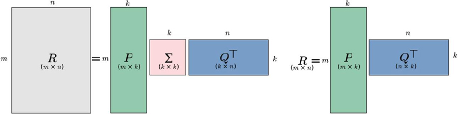
Figure 1 (Left) Dimensionality Reduction with Singular Value Decomposition (SVD). (Right) Dimentionality Reduction with Matrix Factorization (MF) (Sarwar et al., 2000; Ekstrand et al., 2011).
With the truncated SVD recommendation system, user’s and item’s latent spaces are defined respectively by and . In other words, the row of (resp. the column of ) represents the latent factors of user (resp. the latent factors of item ). The reduced latent space can then be used to perform rating-predictions as well as top-N recommendations for users: given user and item , the predicted rating of user on item , denoted by is computed with Equation (9):
| (9) |
Applying SVD for CF recommendation often raises difficulties due to the high portion of missing values caused by sparseness in the user-item ratings matrix. Therefore, to factor the rating matrix, missing values must be filled with reasonable default values (this method is called imputation (Su et al., 2008)). Sarwar et al. (Sarwar et al., 2000) found the item’s mean rating to be a useful default value. Adding ratings normalization by subtracting the user mean rating or other baseline predictor can improve accuracy. The SVD based recommendation algorithm consists of the following steps. Given the rating matrix :
1. Find the normalized rating-matrix ,
2. Factor to obtain matrices , and ,
3. Reduce to dimension to obtain ,
4. Compute the square-root of to obtain ,
5. Compute and that will be used to compute recommendation scores for any user and items.
3.2 Matrix Factorization
The idea behind Matrix Factorization also known as Regularized SVD (Paterek, 2007), is the same as that of the standard SVD: represent users and items in a lower dimensional latent space. The original algorithm4 factorized the user-item rating-matrix as the product of two lower dimensional matrices and , representing latent factors of users and items respectively (see Figure 1.Right). If defines the number of latent factors for users and items, the dimension of and are respectively and . More specifically, each user is associated with a vector and each item with . measure the extent to which item possesses those factors and measure the extent of interest user has in items that have high values on the corresponding factors (Koren et al., 2009; Bokde et al., 2015). Therefore, the dot product of and approximates the user ’s rating on item with defined by Equation (10):
| (10) |
The major challenge lies in computing the mapping of each item and user to factor vectors . After the recommender system completes this mapping, it can easily estimate the rating a user will give to any item (Koren et al., 2009; Parhi et al., 2017). In the training stage, the model includes a regularizer to avoid overfitting. Therefore, the system minimizes the regularized squared error on the set of known ratings. The cost function is defined by Equation (11):
| (11) |
where is the set of the pairs for which is known (the training set) (Paterek, 2007; Koren et al., 2009; Bokde et al., 2015; Zheng et al., 2018). The parameters and control the extent of regularization and is usually determined by cross-validation.
To minimize the cost function , the matrix factorization algorithm computes and the associated error for each training case with the Mean Absolute Error (MAE) metric (Koren et al., 2009). Parameters and are then updated using the stochastic gradient descent algorithm with the following update rules (Equations 12 and 13):
| (12) | |
| (13) |
where is the learning rate. A probabilistic foundation of Matrix Factorization (Probabilistic Matrix Factorization – PMF) is defined in (Mnih and Salakhutdinov, 2008).
3.3 Probabilistic Matrix Factorization (PMF)
Probabilistic algorithms aim to build probabilistic models for user behavior and use those models to predict future behaviors. The core idea of these methods is to compute either the probability that user will purchase item , or the probability that user will rate item (Hofmann, 1999; Ekstrand et al., 2011). These algorithms generally decompose the probability by introducing a set of latent factors and then, decomposes as follows (Equation (14))
| (14) |
where is a latent factor (or feature), the probability that user picks a random feature and the probability to pick a random item given a feature . As illustrated in Figure 2 (left) and detailed in (Hofmann, 1999), a user selects an item by picking the associated factor . This model is known as the Probabilistic Latent Semantic Analysis (PLSA).
The PLSA model has the same form as SVD (Sarwar et al., 2000) or MF (Koren et al., 2009) () except that and are stochastic and not orthogonal. One downside of PLSA is that it’s pretty slow to learn. An alternative probabilistic model is Probabilistic Matrix Factorization (PMF) (Mnih and Salakhutdinov, 2008). With PMF, ratings are drawn from the normal distributions.
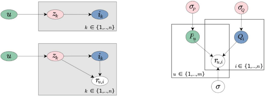
Figure 2 Dimensionality Reduction: Probabilistic Models (Mnih and Salakhutdinov, 2008; Ekstrand et al., 2011). (Left) Probabilistic Latent Semantic Analysis (PLSA). (Right) Probabilistic Matrix Factorization (PMF).
The conditional distribution over the observed ratings (the likelihood term) and the prior distributions over the latent variables and are given by Equations 15, 16 and 17, where the mean for is denoted by (see Figure 2 right).
| (15) | |
| (16) | |
| (17) |
where is the probability density function of the Gaussian distribution with mean and variance , and is the indicator function that is equals to 1 if user rated item and equals to zero otherwise. The complexity of the model is controlled by placing a zero-mean spherical Gaussian priors on and , ensuring that latent variables do not grow too far from zero.
The learning procedure of the Regularized SVD (Matrix Factorization) can be applied to PMF by extending the number of regularization parameters. The goal is to minimize the sum-of-squared-error objective function with quadratic regularization terms (Equation (3.3)):
| (18) |
where , are the regularization parameters and is Frobenius norm. PMF is faster to train than PLSA and showed promising results compared to SVD as experimented in (Mnih and Salakhutdinov, 2008). Despite the effectiveness of PMF, it also has limitations. The basic assumption of PMF is that both users and items are completely independent, while in the field of recommendation, there may be some correlation between different features (Zhang et al., 2018).
3.4 Non-negative Matrix Factorization (NMF)
In MF (Paterek, 2007; Koren et al., 2009) and the PMF (Mnih and Salakhutdinov, 2008) models, values of and are hard to understand, since their components can take arbitrary positive and/or negative values. They do not have any straightforward probabilistic interpretation. Therefore, these models cannot justify the prediction they make since the components of and are difficult to interpret (Hernando et al., 2016).
NMF (Non-negative Matrix Factorization) (Lee and Seung, 1999; Pauca et al., 2006; Cai et al., 2008; Wang and Zhang, 2013; Gillis, 2014; Hernando et al., 2016) is a particular case of Matrix Factorization models where the lower-rank matrices and are non-negative matrices ( and ).
In the NMF model, latent factors with (Lee and Seung, 1999; Cai et al., 2008; Hernando et al., 2016). This allows a probabilistic interpretation: (a) latent factors represent groups of users who share the same interests, (b) the value of represents the probability that user belongs to the group of users and (c) the value represents the probability that users in the group like item . These properties allow the justification of recommendations provided by the NMF model (Lee and Seung, 1999, 2001; Cai et al., 2008; Luo et al., 2014).
The objective function of NMF is equivalent to Equation (11). However, to ensure that the values of and will be kept between 0 and 1, NMF uses multiplicative update rules (equations 21 and 22) (Lee and Seung, 1999, 2001) instead of the additive update rules (Equations 12 and 13). In order to transform additive update rules of the MF model (Equations 12 and 13) into multiplicative ones, Luo et al. (Luo et al., 2014) proposed data-adaptive learning rates (Equation (19)) and (Equation (20)), respectively for and , the idea being to set the learning rate so that any subtraction disappears from the update rules.
| (19) | |
| (20) |
By replacing by in Equation (12) (respectively by in Equation (13)), they obtained multiplicative update rules in Equations 21 and 22 (Luo et al., 2014).
| (21) | |
| (22) |
where is the set of items purchased/rated by user and is the set of users who purchased/rated item . and are the regularizer parameters.
NMF models are also known to be explainable models (Cai et al., 2008; Wang and Zhang, 2013; Luo et al., 2014; Hernando et al., 2016). Indeed, since classical MF models cannot justify their recommendations, justifications or explanations can be added as input to the model in order to provide explainable recommendations.
3.5 Explainable Matrix Factorization (EMF)
In (Abdollahi and Nasraoui, 2017), Abdollahi and Nasraoui proposed an Explainable Matrix Factorization (EMF) model. The proposed model is a probabilistic formulation of their previous EMF model (Abdollahi and Nasraoui, 2016), where the explanation is based on the neighborhood. The neighborhood is either User-based or Item-based (Section 2.2.2). The explainability score (for User-based neighbors style explanation) of the rating of user on item , denoted by is computed with Equation (23) (Abdollahi and Nasraoui, 2017):
| (23) |
where
| (24) |
is the set of users who have given the same rating to item and is the set of -nearest neighbors for user . As you may notice, is the expectation of rating given a set of users. Similarly, for Item-based neighbor style explanation, the explanation score is given by Equation (25).
| (25) |
Finally, the explanation weight of the rating given by user on item is
| (26) |
where is an optimal threshold above which item is considered to be explainable for user . is therefore the extent to which item is explainable for user . The new objective function (Abdollahi and Nasraoui, 2017) can be formulated as in Equation (27):
| (27) |
where is the coefficient of the regularization term and is an explainability regularization coefficient.
Similarity-Based EMF (SEMF) and Neighborhood-based EMF (Wang et al., 2018) are extensions of EMF. In (Wang et al., 2018) the expected value of the explainability score is obtained more reasonably through the Pearson Correlation Coefficient of users or items. SEMF is based on the assumption that if users have a close relationship, the influence of neighbors on users should be larger. Then the high rating items of users who are similar to an active user are also more explainable. Therefore, instead of using the empirical conditional probability of rating as explanation, SEMF uses the Pearson Correlation Coefficient (Resnick et al., 1994). SEMF can be extended over the entire users or items to produce User-based Neighborhood-based EMF or Item-based Neighborhood-based EMF (Wang et al., 2018). Another extension of EMF is Novel and Explainable Matrix Factorization (NEMF) (Coba et al., 2019). This particular model includes novelty information in EMF in order to provide novel and explainable recommendations to users.
3.6 Overview of Dimensionality Reduction Techniques
Matrix Factorization is widely used in rating predictions and can be used to populate the user-element matrix such as that in Tables 1 and 2. Despite the effectiveness of Matrix Factorization models in improving traditional memory-based CF, they are three general issues that arise with this family of models (Shenbin et al., 2020). First, the number of parameters in MF models is huge (): it linearly depends on both the number of users and items, which slows down model learning and may lead to overfitting. Second, making predictions for new users/items based on their ratings implies running optimization procedures in order to find the corresponding user/item embedding. Third, high data sparsity could also lead to overfitting. Moreover, MF models use linear transformations to learn these latent features (Zhang et al., 2019; Shenbin et al., 2020). However, linear models are not complex enough to capture nonlinear patterns from user-item interactions. The learned features are then not sufficiently effective, especially when the rating matrix is highly sparse. Table 4 presents an overview of matrix factorization algorithms.
All of the models explored above (user-based, item-based, and matrix factorization algorithms) are used to predict future interactions between users and products. Using these predictions, it is then possible to populate the score matrices in (for example) Tables 1 and 2 with the missing values and then make recommendations for all users.
Table 4 Overview of Dimensionality Reduction techniques
| Models | Rules |
| Singular Value Decomposition (SVD) (Billsus and Pazzani, 1998; Sarwar et al., 2000) | Decomposes the rating matrix into three low dimensional matrices , and of dimensions , and respectively, where is the rank of the rating matrix, then takes the largest singular values of to yield and reduces and accordingly to obtain and . SVD cannot be applied on a matrix that contains missing values. |
| Regularized SVD (Matrix Factorization) (Paterek, 2007; Koren et al., 2009) | Decomposes into two orthogonal matrices and . It is not necessary to fill missing values before applying Regularized SVD. The learning procedure can be done with gradient descent over all observed ratings. |
| Probabilistic Matrix Factorization (PMF) (Mnih and Salakhutdinov, 2008) | Decomposes into two stochastic matrices and . It assumes that users and items are completely independent and ratings are drawn from the normal distributions. |
| Non-negative Matrix Factorization (NMF) (Lee and Seung, 1999; Cai et al., 2008; Hernando et al., 2016) | Values of and in the MF model are non-interpretable (they can be either positive or negative). NMF restrict values of and between 0 and 1 that allows a probabilistic interpretation of latent factors. |
| Explainable Matrix Factorization (EMF) (Abdollahi and Nasraoui, 2016, 2017; Wang et al., 2018; Coba et al., 2019) | Addresses the explainability of MF in a different way compared to NMF. Here, an item is considered to be explainable for user if a considerable number of user ’s neighbors rated item . |
4 Evaluation Metrics for CF Algorithms
Before applying a recommendation system in real life applications, it is important to measure its aptitude to capture the interest of a particular user in order to provide acceptable recommendations (Bobadilla et al., 2011). The effectiveness of a recommendation system then depends on its ability to measure its own performance and fine-tune the system to do better on test and real data (Breese et al., 1998; Cacheda et al., 2011). However, evaluating recommendation systems and their algorithms is inherently difficult for several reasons: first, different algorithms may be better or worse on different data sets; second, the goals for which an evaluation is performed may differ (Herlocker et al., 2004; Cacheda et al., 2011).
During the two last decades, dozens of metrics have been proposed in order to evaluate the behavior of recommendation systems, from how accurate the system is to how satisfactory recommendations could be. Evaluation metrics can be categorized in four main groups (Herlocker et al., 2004; Cacheda et al., 2011; Bobadilla et al., 2013; Seyednezhad et al., 2018): (a) prediction metrics, such as accuracy (b) set of recommendation metrics, such as precision and recall (c) rank of recommendations metrics like half-life and (d) diversity and novelty.
4.1 Prediction Accuracy
Prediction accuracy measures the difference between the rating the system predicts and the real rating (Cacheda et al., 2011). This evaluation metric is most suitable for the task of rating prediction. Assuming that observed ratings are splitted into train and test sets, prediction accuracy evaluates the ability of the system to behave accurately on the test set. The most popular of these kinds of metrics are Mean Absolute Error (MAE), Mean Squared Error (MSE), Root Mean Squared Error (RMSE) and Normalized Mean Absolute Error (NMAE) (Herlocker et al., 2004; Willmott and Matsuura, 2005; Bobadilla et al., 2011, 2013).
Let us define as the set of users in the recommendation system, as the set of items, the rating of user on item , the lack of rating ( means user has not rated item), the prediction of user on item .
If is the set of items rated by user and having prediction values, we can define the MAE (Equation (28)) and RMSE (Equation (29)) of the system as the average of the user’s MAE and RMSE (Bobadilla et al., 2011, 2013). The prediction’s error is then defined by the absolute difference between prediction and real value .
| (28) | |
| (29) |
Despite their limitations when evaluating systems focused on recommending a certain number of items, the simplicity of their calculations and statistical properties have made MAE and RMSE metrics the most popular when evaluating rating predictions for recommendation systems (Herlocker et al., 2004; Cacheda et al., 2011).
Another important and commonly used metric is coverage, which measures the percentage of items for which the system is able to provide predictions for (Herlocker et al., 2004). The coverage of an algorithm is especially important when the system must find all the good items and not be limited to recommending just a few. According to (Bobadilla et al., 2011, 2013), coverage represents the percentage of situations in which at least one -neighbor of each active user can rate an item that has not been rated yet by that active user. If defines the set of neighbors of user who have rated item , then the coverage of user is defined by Equation (30):
| (30) |
where is the set of items not rated by user but rated by at least one of his -neighbors and the set of items not rated user . The total coverage (Equation (31)) is then defined as the mean of all by:
| (31) |
A high prediction accuracy in a recommendation system doesn’t guarantee the system will provide good recommendations. The confidence of users (or his satisfaction) for a certain recommendation system does not depend directly on the accuracy for the set of possible predictions. A user rather gains confidence on the recommendation system when he agrees with a reduced set of recommendations made by the system (Bobadilla et al., 2011, 2013). Therefore, the most important thing in recommendation systems is not the performance of the system on existing data (products already purchased by users), but rather the performance for future user interactions (products unknown to the user). Moreover, prediction accuracy is suitable when a large number of observed ratings is available, ratings without which training and validation cannot be done effectively. When only a list of items rated by a user is known, it will be preferable to combine prediction accuracy with other evaluation metrics such as Quality of set of recommendations.
4.2 Quality of Set of Recommendations
Quality of set of recommendations is appropriate when a small number of observed ratings is known, and it is used to evaluate the relevance of a set of recommended items (Deshpande and Karypis, 2004). The quality of set of recommendations is usually computed by the following three most popular metrics: (1) Precision, which indicates the proportion of relevant recommended items from the total number of recommended items, (2) Recall, which indicates the proportion of relevant recommended items from the number of relevant items, and (3) F1-score, which is a combination of Precision and Recall (Sarwar et al., 2000; Herlocker et al., 2004; Bobadilla et al., 2011, 2013; Seyednezhad et al., 2018).
Let consider , the set of recommended items to user , the set of relevant items recommended to and its opposite the set of relevant items not recommended to . We consider that an item is relevant for recommendation to user if , where is a threshold.
Assuming that all users accept test recommendations, the evaluations of precision (Equation (32)), recall (Equation (33)) and F1-score (Equation (34)) are obtained by making tests recommendations to the user as follow:
| (32) | |
| (33) | |
| (34) |
One important drawback of this evaluation metric is that all items in a recommendation list are considered equally interesting to a particular user (Desrosiers and Karypis, 2011). However, items in a list of recommendations should be ranked according to the preference of the user. The rank of recommended items is evaluated with the quality of list of recommendations.
4.3 Quality of List of Recommendations
Recommendation systems usually produce lists of items to users. These items are ranked according to their relevance, as users pay more attention to the first recommended items in the list. Errors made on these items are then more serious than those of the last items in the list. The ranking measures consider this situation. The most used metrics for ranking measures are (1) Mean Average Precision (MAP) (Caragea et al., 2009) which is just the mean of the average precision (Equation (32)) over all users, (2) Half-life (Equation (35)) (Breese et al., 1998), which assumes an exponential decrease in the interest of users as they move away from the recommendations at the top and (3) Discounted Cumulative Gain (Equation (36)) (Baltrunas et al., 2010), where the decay is logarithmic:
| (35) | |
| (36) |
where represent the recommended list, the true rating of the user for item , the rank of the evaluated item, the default rating, and the number of the item in the list such that there is a 50% chance the user will review that item.
4.4 Novelty and Diversity
In many applications such as e-commerce, recommendation systems must recommend novel items to users, because companies want to sell their new items as well and keep their clients satisfied. Further, some users may want to explore a new type of item. Therefore, a metric to evaluate recommendation systems based on this criterion would be useful. In this case, we must evaluate the extent to which a recommendation system can produce diverse items. Novelty and diversity are two main metrics that provide such evaluations (Zhang, 2013; Seyednezhad et al., 2018).
The novelty metric evaluates the degree of difference between the items recommended to and known by the user. The novelty of an item (Equation (37)) is measured according to three major criteria: (a) Unknown: is unknown to the user, (b) Satisfactory: is of interest for the user, (c) Dissimilarity: is dissimilar to items in the user’s profile (Zhang, 2013).
| (37) |
where indicates item to item memory-based CF similarity measures and represents the set of recommendations to user .
Novelty is central for recommendation systems, because there are some items which most of the users do not buy frequently (like refrigerators). Thus, if a user buys one of them, most likely he or she will not buy it again in the near future. Then, the recommendation system should not continue to recommend it to the user. However, if the user tries to buy them again, the system should learn that and include them in the set of recommended items (Zhang, 2013; Seyednezhad et al., 2018).
The diversity of a set of recommended items (for example ), indicates the degree of differentiation among recommended items (Bobadilla et al., 2013). It is computed by summing over the similarity between pairs of recommended items and normalizing it (Equation (38)):
| (38) |
Evaluating the diversity and the novelty of a recommendation system ensures that the system will not recommend the same items over and over.
4.5 Overview of Evaluation Metrics
The current main evaluation metrics (detailed previously) are summarized in Table 5.
Table 5 Overview of recommendation system evaluation metrics
| Evaluation Metrics | Measures | Observations |
| Accuracy: useful when a large range of ratings is available. Appropriate for the rating prediction’s task. | – Mean Absolute Error (MEA). – Root Mean Square Error (RMSE). – Coverage: percentage of items that can be recommended. | – Evaluate performances of recommendations over items already purchased (or rated) by users. But we need to know how they will behave on items the user has not purchased yet, – A recommendation system can be highly accurate, but provide poor recommendations. |
| Quality of set of recommendation: users purchased or rated only a few items; Only a small range of ratings is available. Appropriate to recommend good items | – Precision: proportion of relevant recommended items from the total number of recommended items. – Recall: proportion of relevant recommended items from the number of relevant items. – F1-score: combination of precision and recall. | Note: an item is relevant to a user if Where is a threshold – Evaluate the relevance of a set of recommendations provided to a set of users, – Items in the same recommendation list are considered equally interesting to the user. |
| Quality of list of recommendation: rank measure of a list of recommended items. Users give greater importance to the first items recommended to them. This metric Evaluates the utility of a ranked list to the user. | – Half-life (Hl) assume that the interest of a user on the list of recommendations decreases exponentially as we go deeper in the list, – Discounted Cumulative Gain (DCG) the decay here is logarithmic. | Ranking evaluation of the top-N recommendations provided to the user. |
| Novelty and Diversity | – Novelty: evaluate the ability of the system to recommend items not already purchased by users. – Diversity: measure the degree of differentiation among recommended items. | – The goal of a recommendation system is to suggest to a user a set of items that he has not purchased yet. It would be inappropriate to constantly recommend items that the user has already seen. – Diversity is quite important because it ensures that the system won’t recommend all the time the same type of items. |
5 Comparative Experimentation
In this section, we compare performances of all the models previously presented (Sections 2 and 3). We use the MovieLens5 benchmark datasets and evaluate these recommendation algorithms with the MAE evaluation metric (Section 4).
5.1 MovieLens Datasets
The GroupLens Research team6 provides datasets that consist of user ratings (from 1 to 5) on movies. They are various sizes of the MovieLens datasets:
• ML-100K: 100,000 ratings from 1000 users on 1700 movies, released in April 1998,
• ML-1M: 1 million ratings from 6000 users on 4000 movies, released in February 2003,
• ML latest: at the moment we are writing this article, the latest version of the MovieLens dataset contains 27 million ratings applied to 58,000 movies by 280,000 users. The small version of this dataset (MovieLens latest Small) contains 100,000 ratings applied to 9723 movies by 610 users. The latest MovieLens data set changes over time with the same permalink. Therefore, experimental results on this dataset may also change because the distribution of the dataset may change as new versions are released. Therefore, it is not recommended to use the latest small MovieLens dataset for research results. For this reason, we will use only the ML-100K and the ML-1M datasets in our experiments.
In this study we present the experimental testing of the previous models on the ML-100K and the ML-1M datasets and we compare their performances using various evaluation metrics.
5.2 Experimental Results and Performances Comparison
Table 6 presents a performance comparison of User-based and Item-based CF. We use two different datasets and compare the results over the Euclidean and the Cosine-based similarities. The experimental errors of the User-based algorithm with the Cosine distance, 0.75 for ML-100k and 0.73 for ML-1M, is lower than those with the Euclidean distance, 0.81 for both ML-100k and ML-1M. Similarly, the MAEs of the Item-based algorithm with the Cosine distance, 0.51 for ML-100k and 0.42 for ML-1M, is lower than those with the Euclidean distance, 0.83 for ML-100k and 0.82 for ML-1M. Either on the ML-100k dataset or the ML-1M dataset, the Cosine Similarity allows the model to reduce the MAE. This is why the Cosine similarity is generally preferred as a similarity measure compared to the Euclidean distance.
Table 6 User-based vs Item-based performances (MAE) across MovieLens datasets with different similarity-based metrics
| Metric | Dataset | User-based | Item-based |
| Euclidean distance | ML-100k | 0.81 | 0.83 |
| ML-1M | 0.81 | 0.82 | |
| Cosine distance | ML-100k | 0.75 | 0.51 |
| ML-1M | 0.73 | 0.42 |
As stated in Section 2.2.2, Item-based collaborative filtering scales well for online recommendations and globally offer better performances compared to the User-based ones. As described is (Sarwar et al., 2001; Ekstrand et al., 2011), this is due to the fact that items similarities can be calculated in advance, allowing better scaling for online recommendations compared to the User-based algorithm.
5.3 Importance of Ratings Normalization
This section shows the importance of data normalization when training recommendation models. It provides a comparison of the performance of Matrix Factorization models on raw vs normalized ratings. Tables 7 and 8 present results of MF, NMF and EMF with the same number of latent factors and for 10 and 20 epochs respectively.
The MAEs of the MF model on the raw and normalized scores are 1.48 and 0.82, respectively. Normalizing the scores led to an error reduction of 45% from the initial error (on the raw data). To measure the difference between these two values, we performed a t-test with 50 degrees of freedom and obtained a t-value of 3.48 and a p-value of 0.00077 which is far below the classical threshold of 0.05 below which the gap, between 1.48 and 0.82, can be considered significant. This simply means that we have less than a 77 in 100,000 chance of being wrong in stating that this difference is significant.
Table 7 MAE of MF vs. NMF vs. EMF on MovieLens dataset (ML-100k and ML-1M) trained on raw vs. normalized ratings with k=10 over 10 epochs. (a) The introduction of explainable scores leads to better results for the EMF model on each dataset. (b) Due to the non-negativity constraint of the NMF model, it cannot be trained on normalized ratings. (c) Normalization of the data leads to a significant improvement of the MEA
| Metric | Dataset | MF | NMF | EMF |
| Use raw ratings | ML-100k | 1.497 | 0.9510 | 0.797 |
| ML-1M | 1.482 | 0.9567 | 0.76 | |
| Normalized ratings | ML-100k | 0.828 | — | 0.783 |
| ML-1M | 0.825 | — | 0.758 |
Table 8 MAE of MF vs NMF vs EMF on MovieLens dataset trained on raw vs normalized ratings with k=10 on 20 epochs. Compare to Table 7
| Metric | Dataset | MF | NMF | EMF |
| Use raw ratings | ML-100k | 1.488 | 0.868 | 0.784 |
| ML-1M | 1.482 | 0.859 | 0.755 | |
| Normalized ratings | ML-100k | 0.828 | — | 0.78 |
| ML-1M | 0.825 | — | 0.757 |
In the case of EMF, there are no great differences between the MAE errors on raw and normalized ratings (0.78 vs 0.77). This is due to the positive impact of explainable scores that allow the model to reduce biases in the raw ratings leading to better results. The NMF model can only be trained on raw data (it cannot be trained on normalized data). Indeed, normalized data may contain negative values which are not compatible with the non-negativity constraint of the NMF model, reason why we do not have NMF results on normalized data. However, the experimental results in Tables 7 and 8 show the improvement of NMF over MF on raw data.
Based on the results of Tables 7 and 8, we can therefore conclude that normalizing the scores before training MF models leads to a significant reduction of the MAE. Indeed, some users would tend to give higher ratings than others, making their rating scales different and thus incorporating bias into the data (see Section 2.1.2).
Regarding the MAE on raw ratings, we can easily conclude that the EMF model offers better performances (on every dataset) compared to NMF which in turn is better than MF. The performance of EMF over MF and NMF is due to the introduction of explainable scores (Abdollahi and Nasraoui, 2016, 2017; Wang et al., 2018; Coba et al., 2019). Similarly, the performance of NMF over MF is due to the introduction of non-negativity that allows a probabilistic interpretation of latent factors (Lee and Seung, 1999; Cai et al., 2008; Wang and Zhang, 2013; Hernando et al., 2016).
6 Conclusion
In this article, we presented a review on collaborative filtering recommendation systems, with its two majors types: Memory-based CF and Model-based CF. On one hand, Memory-based CF (Section 2), consisting of two main types of algorithms (User-based and Item-based), is highly efficient when ratings are not sparse. However, it cannot handle hight sparsity in user-item data. Moreover, it suffers from scalability concerns due to online computations on huge amounts of data each time a recommendation is needed.
On the other hand, Model-based recommendation systems (Section 3) have been designed to address the limitations of their memory-based counterparts. In this article we focused essentially on Dimensionality Reduction models. Several such methods have been covered: Matrix Factorization (MF), Non-negative Matrix Factorization (NMF) and Explainable Matrix Factorization (EMF). These models appear as the most important ones in Dimensionality Reduction, due to their ability to capture user’s preferences through latent factors. To complete further our analysis, our experimentation on the MovieLens benchmark dataset (Section 4) illustrates that due to its non-negativity, the NMF model offers better performance that MF. On the other hand, EMF offers better performance that MF and NMF due to the introduction of explainable score. We did our experimentation on the ML-100K benchmark dataset. The source code of our experimentation is available on github (Section 7).
Future Works
We have reviewed that in the EMF model, the explainable scores are included in the MF model, which leads to better results (see Table 7) compared to MF and NMF. However, due to the use of the additive update rules, the latent factors and of the EMF model may still contain negative values that are not interpretable. We also reviewed that applying non-negativity to the MF model, to produce the NMF model, yields higher performances of recommendations due to the probability interpretation of the latent factors. We have therefore formulated the following hypotheses: Since applying non-negativity to the MF model led to better results, introducing non-negativity to the EMF model will further improve the recommendation performance compare to MF, NMF and EMF. The resultant model will be a two-stage explainable model: (a) the probabilistic interpretation of latent factors and (b) the further explainability with explainable weights. Designing such a Non-negative Explainable Matrix Factorization (NEMF) is a research direction we are exploring.
Due to space limitation, we have not included the deep learning recommendation systems in this paper. A thorough study of these models is the subject of our future work.
7 Resources
All experiments have been made with Python 3.7 on the Jupyter notebook with Intel Core i5, 7th gen (2.5GHz) and 8Go RAM.
Requirements
Matplotlib==3.2.2; Numpy == 1.19.2; Pandas == 1.0.5; Scikit-learn == 0.24.1; Scikit-surprise == 1.1.1; Scipy == 1.6.2
Github Repository
Our experiments are available on the following github repository: https://github.com/nzhinusoftcm/review-on-collaborative-filtering/. The repository contains the following notebooks:
– User-based Collaborative Filtering: implements the User-based recommendation system. https://github.com/nzhinusoftcm/review-on-collaborative-filtering/blob/master/2.User-basedCollaborativeFiltering.ipynb
– Item-based Collaborative Filtering: implements the Item-based recommendation system. https://github.com/nzhinusoftcm/review-on-collaborative-filtering/blob/master/3.Item-basedCollaborativeFiltering.ipnb
– Matrix Factorization: implements the Matrix Factorization Model: https://github.com/nzhinusoftcm/review-on-collaborative-filtering/blob/master/5.MatrixFactorization.ipynb
– Non-negative Matrix Factorization: implements the Non-negative Matrix Factorization model. https://github.com/nzhinusoftcm/review-on-collaborative-filtering/blob/master/6.NonNegativeMatrixFactorization.ipynb
– Explainable Matrix Factorization: implements the Explainable Matrix Factorization model: https://github.com/nzhinusoftcm/review-on-collaborative-filtering/blob/master/7.ExplainableMatrixFactorization.ipynb
– Performance measure: https://github.com/nzhinusoftcm/review-on-collaborative-filtering/blob/master/8.PerformancesMeasure.ipynb
Notebooks with Google Collaboratory
To run these notebooks with Google Collaboratory, we provide the following link. https://colab.research.google.com/github/nzhinusoftcm/review-on-collaborative-filtering/
Footnotes
1Numpy/Pandas implementation of models presented in this paper (https://github.com/nzhinusoftcm/review-on-collaborative-filtering)
2MovieLens (https://grouplens.org/datasets/movielens/) is a benchmark dataset collected and made available in several sizes (100k, 1M, 25M) by the GroupLens Research team.
3The Netflix Price (https://netflixprize.com) sought to substantially improve the accuracy of predictions about how much someone is going to enjoy a movie based on their movie preferences.
4Funk, S (2006). Netflix Update: Try This at Home. https://sifter.org/~simon/journal/20061211.html
5MovieLens (https://movielens.org/) is a web-based recommendation system and virtual community that recommends movies to its users, based on their past preferences using collaborative filtering.
6GroupLens Research (https://grouplens.org/) is a research laboratory from the University of Minnesota, that advances the theory and practice of social computing by building and understanding systems used by real people.
References
Abdollahi and Nasraoui (2016) Abdollahi, B., and O. Nasraoui, 2016: Explainable matrix factorization for collaborative filtering. Proceedings of the 25th International Conference Companion on World Wide Web, International World Wide Web Conferences Steering Committee, Republic and Canton of Geneva, CHE, 5–6, WWW ’16 Companion, URL https://doi.org/10.1145/2872518.2889405.
Abdollahi and Nasraoui (2017) Abdollahi, B., and O. Nasraoui, 2017: Using explainability for constrained matrix factorization. Proceedings of the Eleventh ACM Conference on Recommender Systems, ACM, New York, NY, USA, URL https://doi.org/10.1145/3109859.3109913.
Ali and Majeed (2021) Ali, S. I. M., and S. S. Majeed, 2021: A review of collaborative filtering recommendation system. Almuthanna Journal of Pure Science (MJPS), 8, 120–131, doi:10.52113/2/08.01.2021/120-131.
Ansari et al. (2000) Ansari, A., S. Essegaier, and R. Kohli, 2000: Internet recommendation systems. J. Mark. Res., 37 (3), 363–375, URL http://dx.doi.org/10.1509/jmkr.37.3.363.18779.
Baltrunas et al. (2010) Baltrunas, L., T. Makcinskas, and F. Ricci, 2010: Group recommendations with rank aggregation and collaborative filtering. Proceedings of the fourth ACM conference on Recommender systems, Association for Computing Machinery, New York, NY, USA, 119–126, RecSys ’10, URL https://doi.org/10.1145/1864708.1864733.
Billsus and Pazzani (1998) Billsus, D., and M. J. Pazzani, 1998: Learning collaborative information filters. Proceedings of the Fifteenth International Conference on Machine Learning (ICML 1998), Madison, Wisconsin, USA, July 24-27, 1998, J. W. Shavlik, Ed., Morgan Kaufmann, 46–54.
Bobadilla et al. (2011) Bobadilla, J., A. Hernando, F. Ortega, and J. Bernal, 2011: A framework for collaborative filtering recommender systems. Expert Syst. Appl., 38 (12), 14 609–14 623, URL https://doi.org/10.1016/j.eswa.2011.05.021.
Bobadilla et al. (2013) Bobadilla, J., F. Ortega, A. Hernando, and A. Gutiérrez, 2013: Recommender systems survey. Knowledge-Based Systems, 46, 109–132, URL https://doi.org/10.1016/j.knosys.2013.03.012.
Bokde et al. (2015) Bokde, D., S. Girase, and D. Mukhopadhyay, 2015: Matrix factorization model in collaborative filtering algorithms: A survey. Procedia Comput. Sci., 49, 136–146, URL https://doi.org/10.1016/j.procs.2015.04.237.
Breese et al. (1998) Breese, J. S., D. Heckerman, and C. Kadie, 1998: Empirical analysis of predictive algorithms for collaborative filtering. Proceedings of the Fourteenth Conference on Uncertainty in Artificial Intelligence, Morgan Kaufmann Publishers Inc., San Francisco, CA, USA, 43–52, UAI’98, URL https://arxiv.org/abs/1301.7363.
Cacheda et al. (2011) Cacheda, F., V. Carneiro, D. Fernández, and V. Formoso, 2011: Comparison of collaborative filtering algorithms: Limitations of current techniques and proposals for scalable, high-performance recommender systems. ACM Trans. Web, 5 (1), 1–33, URL https://doi.org/10.1145/1921591.1921593.
Cai et al. (2008) Cai, D., X. He, X. Wu, and J. Han, 2008: Non-negative matrix factorization on manifold. Proceedings – 8th IEEE International Conference on Data Mining, ICDM 2008, 63–72, Proceedings – IEEE International Conference on Data Mining, ICDM, doi:10.1109/icdm.2008.57, URL https://doi.org/10.1109/ICDM.2008.57, copyright: Copyright 2012 Elsevier B.V., All rights reserved.; 8th IEEE International Conference on Data Mining, ICDM 2008 ; Conference date: 15-12-2008 Through 19-12-2008.
Caragea et al. (2009) Caragea, C., and Coauthors, 2009: Mean average precision. Encyclopedia of Database Systems.
Chee et al. (2001) Chee, S. H. S., J. Han, and K. Wang, 2001: RecTree: An efficient collaborative filtering method. Data Warehousing and Knowledge Discovery, Lecture notes in computer science, Springer Berlin Heidelberg, Berlin, Heidelberg, 141–151, URL https://doi.org/10.1007/3-540-44801-2“˙15.
Coba et al. (2019) Coba, L., P. Symeonidis, and M. Zanker, 2019: Personalised novel and explainable matrix factorisation. Data Knowl. Eng., 122, 142–158, URL https://doi.org/10.1016/j.datak.2019.06.003.
Deerwester et al. (1990) Deerwester, S., S. T. Dumais, G. W. Furnas, T. K. Landauer, and R. Harshman, 1990: Indexing by latent semantic analysis. J. Am. Soc. Inf. Sci., 41 (6), 391–407.
Deshpande and Karypis (2004) Deshpande, M., and G. Karypis, 2004: Item-based top- N recommendation algorithms. ACM Trans. Inf. Syst. Secur., 22 (1), 143–177, URL https://doi.org/10.1145/963770.963776.
Desrosiers and Karypis (2011) Desrosiers, C., and G. Karypis, 2011: A comprehensive survey of neighborhood-based recommendation methods. Recommender Systems Handbook, F. Ricci, L. Rokach, B. Shapira, and P. B. Kantor, Eds., Springer US, Boston, MA, 107–144, doi:10.1007/978-0-387-85820-3˙4, URL http://dx.doi.org/10.1007/978-0-387-85820-3˙4.
Dillon (1983) Dillon, M., 1983: Introduction to modern information retrieval. Inf. Process. Manag., 19 (6), 402–403.
Ekstrand et al. (2011) Ekstrand, M. D., J. T. Riedl, and J. A. Konstan, 2011: Collaborative filtering recommender systems. Foundations and Trends® in Human–Computer Interaction, 4 (2), 81–173, URL https://doi.org/10.1561/1100000009.
Feigl and Bogdan (2017) Feigl, J., and M. Bogdan, 2017: Collaborative filtering with neural networks. ESANN, URL http://www.elen.ucl.ac.be/Proceedings/esann/esannpdf/es2017-23.pdf.
Gillis (2014) Gillis, N., 2014: The why and how of nonnegative matrix factorization. Regularization, Optimization, Kernels, and Support Vector Machines, URL http://arxiv.org/abs/1401.5226.
Goldberg et al. (1992) Goldberg, D., D. Nichols, B. M. Oki, and D. Terry, 1992: Using collaborative filtering to weave an information tapestry. Commun. ACM, 35 (12), 61–70, URL https://doi.org/10.1145/138859.138867.
Goldberg et al. (2001) Goldberg, K., T. Roeder, D. Gupta, and C. Perkins, 2001: Eigentaste: A constant time collaborative filtering algorithm. Inf. Retr. Boston., 4, 133–151, URL https://doi.org/10.1023/A:1011419012209.
He et al. (2018) He, X., X. Du, X. Wang, F. Tian, J. Tang, and T. Chua, 2018: Outer product-based neural collaborative filtering. Proceedings of the Twenty-Seventh International Joint Conference on Artificial Intelligence, IJCAI 2018, July 13-19, 2018, Stockholm, Sweden, J. Lang, Ed., ijcai.org, 2227–2233, doi:10.24963/ijcai.2018/308, URL https://doi.org/10.24963/ijcai.2018/308.
He et al. (2017a) He, X., L. Liao, H. Zhang, L. Nie, X. Hu, and T. Chua, 2017a: Neural collaborative filtering. Proceedings of the 26th International Conference on World Wide Web, WWW 2017, Perth, Australia, April 3-7, 2017, R. Barrett, R. Cummings, E. Agichtein, and E. Gabrilovich, Eds., ACM, 173–182, doi:10.1145/3038912.3052569, URL https://doi.org/10.1145/3038912.3052569.
He et al. (2017b) He, X., L. Liao, H. Zhang, L. Nie, X. Hu, and T.-S. Chua, 2017b: Neural collaborative filtering. Proceedings of the 26th International Conference on World Wide Web, International World Wide Web Conferences Steering Committee, Republic and Canton of Geneva, CHE, 173–182, WWW ’17, URL https://doi.org/10.1145/3038912.3052569.
Herlocker et al. (1999) Herlocker, J. L., J. A. Konstan, A. Borchers, and J. Riedl, 1999: An algorithmic framework for performing collaborative filtering. Proceedings of the 22nd annual international ACM SIGIR conference on Research and development in information retrieval, Association for Computing Machinery, New York, NY, USA, 230–237, SIGIR ’99, URL https://doi.org/10.1145/312624.312682.
Herlocker et al. (2004) Herlocker, J. L., J. A. Konstan, L. G. Terveen, and J. T. Riedl, 2004: Evaluating collaborative filtering recommender systems. ACM Trans. Inf. Syst. Secur., 22 (1), 5–53, URL https://doi.org/10.1145/963770.963772.
Hernando et al. (2016) Hernando, A., J. Bobadilla, and F. Ortega, 2016: A non negative matrix factorization for collaborative filtering recommender systems based on a bayesian probabilistic model. Knowledge-Based Systems, 97, 188–202, URL https://doi.org/10.1016/j.knosys.2015.12.018.
Hofmann (1999) Hofmann, T., 1999: Probabilistic latent semantic indexing. Proceedings of the 22nd annual international ACM SIGIR conference on Research and development in information retrieval – SIGIR ’99, ACM Press, New York, New York, USA, URL https://doi.org/10.1145/312624.312649.
Hu and Li (2018) Hu, J., and P. Li, 2018: Collaborative filtering via additive ordinal regression. Proceedings of the Eleventh ACM International Conference on Web Search and Data Mining, Association for Computing Machinery, New York, NY, USA, 243–251, WSDM ’18, URL https://doi.org/10.1145/3159652.3159723.
Karypis (2001) Karypis, G., 2001: Evaluation of Item-Based Top-N recommendation algorithms. Proceedings of the tenth international conference on Information and knowledge management, Association for Computing Machinery, New York, NY, USA, 247–254, CIKM ’01, URL https://doi.org/10.1145/502585.502627.
Khalifeh and Al-Mousa (2021) Khalifeh, S., and A. A. Al-Mousa, 2021: A book recommender system using collaborative filtering method. DATA’21: International Conference on Data Science, E-learning and Information Systems 2021, Petra, Jordan, 5-7 April, 2021, J. A. L. Torralbo, S. A. Aljawarneh, V. Radhakrishna, and A. N., Eds., ACM, 131–135, doi:10.1145/3460620.3460744, URL https://doi.org/10.1145/3460620.3460744.
Koren et al. (2009) Koren, Y., R. Bell, and C. Volinsky, 2009: Matrix factorization techniques for recommender systems. Computer, 42 (8), 30–37, URL https://doi.org/10.1109/MC.2009.263.
Kunegis and Albayrak (2007) Kunegis, J., and S. Albayrak, 2007: Adapting ratings in Memory-Based collaborative filtering using linear regression. 2007 IEEE International Conference on Information Reuse and Integration, 49–54, URL https://doi.org/10.1109/IRI.2007.4296596.
Lakshminarayanan et al. (2011) Lakshminarayanan, B., G. Bouchard, and C. Archambeau, 2011: Robust bayesian matrix factorisation. Proceedings of the Fourteenth International Conference on Artificial Intelligence and Statistics, 425–433, URL http://proceedings.mlr.press/v15/lakshminarayanan11a/lakshminarayanan11a.pdf.
Lee and Seung (2001) Lee, D., and H. Seung, 2001: Algorithms for non-negative matrix factorization. Advances in Neural Information Processing Systems 13 – Proceedings of the 2000 Conference, NIPS 2000, 13.
Lee and Seung (1999) Lee, D. D., and H. S. Seung, 1999: Learning the parts of objects by non-negative matrix factorization. Nature, 401, 788–791, doi:10.1038/44565, URL https://doi.org/10.1038/44565.
Linden et al. (2003) Linden, G., B. Smith, and J. York, 2003: Amazon.com recommendations: item-to-item collaborative filtering. IEEE Internet Comput., 7 (1), 76–80, URL https://doi.org/10.1109/MIC.2003.1167344.
Luo et al. (2014) Luo, X., M. Zhou, Y. Xia, and Q. Zhu, 2014: An efficient non-negative matrix-factorization-based approach to collaborative filtering for recommender systems. IEEE Trans. Ind. Informatics, 10 (2), 1273–1284, doi:10.1109/TII.2014.2308433, URL https://doi.org/10.1109/TII.2014.2308433.
Mild and Natter (2002) Mild, A., and M. Natter, 2002: Collaborative filtering or regression models for internet recommendation systems? Journal of Targeting, Measurement and Analysis for Marketing, 10 (4), 304–313, URL http://dx.doi.org/10.1057/palgrave.jt.5740055.
Mnih and Salakhutdinov (2008) Mnih, A., and R. R. Salakhutdinov, 2008: Probabilistic matrix factorization. Advances in Neural Information Processing Systems, J. Platt, D. Koller, Y. Singer, and S. Roweis, Eds., Curran Associates, Inc., Vol. 20, 1257–1264.
Mu (2018) Mu, R., 2018: A survey of recommender systems based on deep learning. IEEE Access, 6, 69 009–69 022, URL https://doi.org/10.1109/ACCESS.2018.2880197.
Parhi et al. (2017) Parhi, P., A. Pal, and M. Aggarwal, 2017: A survey of methods of collaborative filtering techniques. 2017 International Conference on Inventive Systems and Control (ICISC), 1–7, URL http://dx.doi.org/10.1109/ICISC.2017.8068603.
Paterek (2007) Paterek, A., 2007: Improving regularized singular value decomposition for collaborative filtering. Proceedings of KDD cup and workshop, Vol. 2007, 5–8, URL https://www.cs.uic.edu/~liub/KDD-cup-2007/proceedings/Regular-Paterek.pdf.
Pauca et al. (2006) Pauca, V. P., J. Piper, and R. J. Plemmons, 2006: Nonnegative matrix factorization for spectral data analysis. Linear Algebra and its Applications, 416 (1), 29–47, URL https://doi.org/10.1016/j.laa.2005.06.025, special Issue devoted to the Haifa 2005 conference on matrix theory.
Pazzani and Billsus (2007) Pazzani, M. J., and D. Billsus, 2007: Content-Based recommendation systems. The Adaptive Web: Methods and Strategies of Web Personalization, P. Brusilovsky, A. Kobsa, and W. Nejdl, Eds., Springer Berlin Heidelberg, Berlin, Heidelberg, 325–341.
Rawat and Wang (2017) Rawat, W., and Z. Wang, 2017: Deep convolutional neural networks for image classification: A comprehensive review. Neural Computation, 29 (9), 2352–2449, URL https://doi.org/10.1162/NECO˙a˙00990.
Resnick et al. (1994) Resnick, P., N. Iacovou, M. Suchak, P. Bergstrom, and J. Riedl, 1994: GroupLens: an open architecture for collaborative filtering of netnews. Proceedings of the 1994 ACM conference on Computer supported cooperative work, Association for Computing Machinery, New York, NY, USA, 175–186, CSCW ’94, URL https://doi.org/10.1145/192844.192905.
Sarwar et al. (2000) Sarwar, B., G. Karypis, J. Konstan, and J. Riedl, 2000: Application of dimensionality reduction in recommender system: A case study. Computer Science and Engineering (CS E) Technical Reports, URL https://hdl.handle.net/11299/215429.
Sarwar et al. (2001) Sarwar, B. M., G. Karypis, J. A. Konstan, and J. Riedl, 2001: Item-based collaborative filtering recommendation algorithms. Proceedings of the Tenth International World Wide Web Conference, WWW 10, Hong Kong, China, May 1-5, 2001, V. Y. Shen, N. Saito, M. R. Lyu, and M. E. Zurko, Eds., ACM, 285–295, doi:10.1145/371920.372071, URL https://doi.org/10.1145/371920.372071.
Saxena et al. (2017) Saxena, A., and Coauthors, 2017: A review of clustering techniques and developments. Neurocomputing, 267, 664–681, URL https://doi.org/10.1016/j.neucom.2017.06.053.
Sedhain et al. (2015) Sedhain, S., A. K. Menon, S. Sanner, and L. Xie, 2015: AutoRec: Autoencoders meet collaborative filtering. Proceedings of the 24th International Conference on World Wide Web, Association for Computing Machinery, New York, NY, USA, 111–112, WWW ’15 Companion, URL https://doi.org/10.1145/2740908.2742726.
Seyednezhad et al. (2018) Seyednezhad, S. M. M., K. N. Cozart, J. A. Bowllan, and A. O. Smith, 2018: A review on recommendation systems: Context-aware to social-based. CoRR, abs/1811.11866, URL http://arxiv.org/abs/1811.11866, 1811.11866.
Shenbin et al. (2020) Shenbin, I., A. Alekseev, E. Tutubalina, V. Malykh, and S. I. Nikolenko, 2020: RecVAE: A new variational autoencoder for Top-N recommendations with implicit feedback. Proceedings of the 13th International Conference on Web Search and Data Mining, Association for Computing Machinery, New York, NY, USA, 528–536, WSDM ’20, URL https://doi.org/10.1145/3336191.3371831.
Srifi et al. (2020) Srifi, M., A. Oussous, A. Ait Lahcen, and S. Mouline, 2020: Recommender systems based on collaborative filtering using review texts—a survey. Information, 11 (6), doi:10.3390/info11060317, URL https://www.mdpi.com/2078-2489/11/6/317.
Steck (2019) Steck, H., 2019: Collaborative filtering via High-Dimensional regression. ArXiv, abs/1904.13033, URL http://arxiv.org/abs/1904.13033, 1904.13033.
Su and Khoshgoftaar (2009) Su, X., and T. M. Khoshgoftaar, 2009: A survey of collaborative filtering techniques. Advances in Artificial Intelligence, 2009, URL https://doi.org/10.1155/2009/421425.
Su et al. (2008) Su, X., T. M. Khoshgoftaar, X. Zhu, and R. Greiner, 2008: Imputation-boosted collaborative filtering using machine learning classifiers. Proceedings of the 2008 ACM symposium on Applied computing, Association for Computing Machinery, New York, NY, USA, 949–950, SAC ’08, URL https://doi.org/10.1145/1363686.1363903.
Ungar and Foster (1998) Ungar, L. H., and D. P. Foster, 1998: Clustering methods for collaborative filtering. AAAI workshop on recommendation systems, Vol. 1, 114–129, URL https://www.aaai.org/Papers/Workshops/1998/WS-98-08/WS98-08-029.pdf.
Vucetic and Obradovic (2005) Vucetic, S., and Z. Obradovic, 2005: Collaborative filtering using a Regression-Based approach. Knowl. Inf. Syst., 7 (1), 1–22, URL https://doi.org/10.1007/s10115-003-0123-8.
Wang et al. (2018) Wang, S., H. Tian, X. Zhu, and Z. Wu, 2018: Explainable matrix factorization with constraints on neighborhood in the latent space. Data Mining and Big Data, Lecture notes in computer science, Springer International Publishing, Cham, 102–113, URL http://dx.doi.org/10.1007/978-3-319-93803-5˙10.
Wang and Zhang (2013) Wang, Y., and Y. Zhang, 2013: Nonnegative matrix factorization: A comprehensive review. IEEE Trans. Knowl. Data Eng., 25 (6), 1336–1353, URL https://doi.org/10.1109/TKDE.2012.51.
Willmott and Matsuura (2005) Willmott, C., and K. Matsuura, 2005: Advantages of the mean absolute error (mae) over the root mean square error (rmse) in assessing average model performance. Climate Research, 30, 79, doi:10.3354/cr030079, URL https://doi.org/10.3354/cr030079.
Xu and Tian (2015) Xu, D., and Y. Tian, 2015: A comprehensive survey of clustering algorithms. Annals of Data Science, 2 (2), 165–193, URL https://doi.org/10.1007/s40745-015-0040-1.
Yu et al. (2019) Yu, Y., X. Si, C. Hu, and J. Zhang, 2019: A review of recurrent neural networks: LSTM cells and network architectures. Neural Compution, 31 (7), 1235–1270, URL https://doi.org/10.1162/neco˙a˙01199.
Zhang (2013) Zhang, L., 2013: The definition of novelty in recommendation system. J. Eng. Sci. Technol. Rev., 6 (3), 141–145, URL http://dx.doi.org/10.25103/jestr.063.25.
Zhang et al. (2018) Zhang, L., T. Luo, F. Zhang, and Y. Wu, 2018: A recommendation model based on deep neural network. IEEE Access, 6, 9454–9463, URL https://doi.org/10.1109/ACCESS.2018.2789866.
Zhang et al. (2019) Zhang, S., L. Yao, A. Sun, and Y. Tay, 2019: Deep learning based recommender system: A survey and new perspectives. ACM Comput. Surv., 52 (1), 1–38, URL https://doi.org/10.1145/3285029.
Zheng et al. (2018) Zheng, S., C. Ding, and F. Nie, 2018: Regularized singular value decomposition and application to recommender system. ArXiv, URL http://arxiv.org/abs/1804.05090, 1804.05090.
Biographies

Carmel Wenga is a PhD student at the University of French Polynesia. He obtained his master’s degree in Networks and Distributed Systems, his main field is machine learning applied to recommender systems. He is an active member of the NzhinuSoft research team and is actively involved in the development of the recommendation system of ShoppingList, an e-commerce application of NzhinuSoft and deployed in Cameroon. He also works as a Data Engineering & Middleware Developer Consultant for NzhinuSoft.

Majirus Fansi is Software Architect and CEO at NzhinSoft. He Holds a PhD in computer science from Université de Pau et des Pays de l’Adour and a MBA degree from Stockholm Business School. He has founded NzhinuSoft, on the promise of valorizing enterprise data through data engineering, Data Science, data Visualization, and Application development. His current research interest is recommender systems based on images. First results are implemented on shoppinglist.cm, a market place developed by NzhinuSoft.

Sébastien Chabrier is Associate Professor in Computer Science at the University of French Polynesia working on image processing and machine learning. In year 2003 he received his PhD in image processing and machine learning and in 2021 his French “Habilitation to Lead Research” (HDR) from the University of French Polynesia.

Jean-Martial Mari is Associate Professor in Computer Science at the University of French Polynesia working on signal and image processing. In year 2000 he received the Electrical Engineering diploma of the INSA Lyon, France, with a specialization in Signal Processing, and a Master degree (DEA) in signal and image processing. In 2004 he received his PhD in Acoustics and in 2012 his French “Habilitation to Lead Research” (HDR) from the Université Claude Bernard Lyon 1 (France).

Alban Gabillon is a full Professor of computer science at the University of French Polynesia. His main research interests are in computer security since his PhD thesis in 1995. He has more recently diversified his activities in the field of machine learning. He is the author or co-author of more than 100 research papers.
Journal of Machine Learning Theory, Applications and Practice, Vol. 1, 1–44.
doi: 10.13052/jmltapissn.2023.001
This is an Open Access publication. © 2023 the Author(s). All rights reserved.