A Greedy Reconstruction Heuristic for Solving the Minimum Travelling Salesman Tour Problem
Santosh Kumar1,* OAM and Elias Munapo2
1Department of Mathematical and Geospatial Sciences, School of Sciences, RMIT University, Melbourne Australia
2School of Economics and Decision Sciences, North West University, Mafikeng 2735, South Africa
E-mail: Santosh.Kumarau@gmail.com; Santosh.Kumar@rmit.edu.au; emunapo@gmail.com; Elias.Munapo@nwu.ac.za
*Corresponding Author
Nearest neighbour approach for determination of the minimum travelling salesman tour is a well-documented heuristic for a quick identification of the salesman tour and its associated cost. This heuristic has been used on large sized networks for a quick approximate solution to the travelling salesman problem. For the last several years, an alternative approach to the minimum travelling salesman tour has been developed through the minimum spanning tree (MST). The MST was converted to an index restricted MST (IRMST) and that IRMST was used to find the minimum travelling salesman tour. These two approaches, i.e., the greedy heuristics and the index restricted minimum spanning tree seems to have stronger relations and it is this relationship, which has been explored in this paper. The nearest neighbour approach to find the travelling salesman tour has been modified by incorporating the index balancing theorem. A further modification to this heuristic has been suggested to identify the minimum travelling salesman tour. Many small size problems have been attempted using the heuristic discussed in this paper, and it resulted in an optimal solution but an analytical proof for optimality remains a challenge. This approach further strengthens a natural question about the ‘NP Hard’ category associated with the minimum travelling salesman tour problem.
Keywords: Travelling salesman tour, shortest connected graph, index restricted shortest connected graph, travelling salesman heuristic, nearest-neighbour heuristic to the travelling salesman.
From time to time, the mathematics of OR has provided analytical tools or heuristics for resolving real-life industrial and business decision-making situations. Some of these situations can be represented in the form of a network, and appropriate network tools have been used for resolving those situations. In general, a network is represented by , where represents a set of entities denoted by the nodes and is the set of links joining various pair of nodes. The weights associated with links represent a quantitative measure of properties associated with these pair of nodes. Links are denoted by , where and are the nodes and . In a weighted network, each link is assigned a weight providing that quantitative measure of the relationship between the pair of nodes. Let the weight associated with the link be denoted by , which can be a positive or a negative quantity, depending on the situation and its physical interpretation of the relationship.
Kumar and Munapo in [1] considered a few classical network routing problems, and based on them developed some innovative ways to create alternatives in different situations and used those alternatives to solve some difficult combinatorial network optimization problems. The travelling salesman problem was one of these problems discussed in that paper. They approached the travelling salesman problem through the minimum connected tree approach. The minimum connected tree (MCT) and its variation in the form of index restricted minimum connected tree (IRMCT) has a strong relation with the minimum travelling salesman tour. This earlier work by the authors has been reviewed in Section 2. The nearest-neighbour heuristic is briefly presented in Section 3, and a heuristic, incorporating the index balancing theorem, for the travelling salesman problem has been discussed in Section 4. In Section 5, we again approach the travelling salesman problem as an index restricted minimum connected tree for a reconstructed network and find the minimum travelling salesman tour. In this approach, the index restricted path and the minimum travelling salesman tour are equivalent, hence results in an optimal solution. Numerical examples have been discussed in Sections 4 and 5 to illustrate approaches discussed in those sections. Finally, the paper is concluded with some remarks in Section 6.
The travelling salesman problem has received much attention, and researchers have developed analytical as well as heuristic approaches, see Nemhauser and Wolsey [2]. In this section, we briefly review some work on the travelling salesman problem that is based on the shortest connected graph of a given network. Since the shortest connected network can be obtained by a greedy approach, these approaches have raised a natural question about the ‘NP Hard’ category assigned to the travelling salesman problem. These approaches for the travelling salesman problem were mainly developed by the authors and their associates, see [3–5].
The minimum travelling salesman tour is a classical graph theory problem, where the aim is to find the minimum cost tour passing through all nodes of the network once and return to the home city. This classical travelling salesman problem has lot of industrial applications, and it has been classified as a ‘NP Hard’ problem, see [1, 2, 6]. In [7] Christofides has discussed worst-case ratio of the heuristic for the travelling salesman problem, and established that ration is .
The shortest connected network (SCN) is also a classical network theory problem that has been attempted by the greedy approach, see [8–10]. These two problems connect all nodes of the given network with different objectives. For example, in the case of TSP, the objective is to find the minimum cost tour that starts from a given node and returns to the same node after visiting each node once in minimum total cost. In the case of SCN, aim is to connect all nodes with minimum total cost. A network, , consists of nodes representing the entities, and links joining various pairs of nodes. Each link , is assigned a link weight , where and are the nodes and . In a ‘’ node connected network, the minimum salesman tour is comprised of n links, which start from any given node and returns to the same node after visiting all other nodes once and total cost is minimum. The minimum spanning tree of the network is comprised of links which form a tree of the given set of nodes and total weight of the selected links is minimum. These two problems dealing with all nodes of the network have some intimate relations. One of these relationships is in the form of an index restricted connected tree was investigated by Munapo et al. in [11]. The index restricted shortest connected network (IRSCN) is a slight modification of the conventional shortest connected network. In the IRSCN, the index for nodes are restricted to 2, and for the remaining two nodes, the index is restricted to 1. Therefore, the IRSCN of links form a path joining two single index nodes passing through all the remaining nodes. Suppose a link, that has not been used for this path is selected to join these two single index nodes, it will form a feasible travelling salesman tour, hence its total length can be seen as an upper bound on the required minimum travelling salesman tour. This relationship between the IRSCN and the minimum cost TST problem has been investigated by in [3, 4] and finally the minimum spanning tree under the index restriction was established equal to the minimum travelling salesman tour, see [1, 5]. Some other relevant references are [12–14, 17–19].
The shortest connected network (SCN) of is comprised of links. These links are selected by the greedy approach, see [8–10]. Here ‘n’ represents the number of nodes in the given network . The SCN has a unique path from every node to every other node, and that path is free of loops. In such a SCN network, if any link is removed, it will result in a disconnect network. If an additional link is added, it forms a loop. A modification of the SCN was proposed by Munapo et al. in [11], which is briefly reviewed in Section 2.2.
For a given , the SCN can be obtained by any known method, and node index values for each node can be identified. If the node index of the node is represented by , each node in the SCN will satisfy the condition , whereas the index restricted shortest connected network requires each node, other than the source and the destination node to satisfy . The index of the source and the destination node is 1. It means the SCN must be modified to satisfy the condition . The IRSCN forms a path joining two nodes and passing through all other remaining nodes of the network.
Shape of the IRSCN: Each selected link generates two indices, the total number of indices of the selected links forming the SCN will be . Alternatively, a path joining two nodes and passing through all other remaining nodes, will also have a total index value .
High and low index nodes: Once a SCN of the given has been identified by using any known method, with index value . These index values must be changed to satisfy the condition , i.e., for the origin and the destination nodes the , and for all other remaining (n-2) nodes, . High index nodes will be the nodes where the current index value is higher than required.
Adding the same constant to all links emanating from the same node does not change the relative merit of any given selected link in the SCN obtained by the greedy approach. However, an appropriate constant when added to all links emanating from the same node can create an alternative. Since in the given SCN, low and high index nodes are known, the index balancing theorem is used reduce the index value of a high index node by adding constants to all links that are emanating from that high index node. The idea is to create an alternative for the selection of a link and reduce index at a high index node and increases the index of a low index node. It is done by removing a link from a high index node and place that link between two low index nodes. This process can be repeated, until all nodes attain the required index and satisfy all index restrictions as required by the IRSCN.
In this paper, we apply this index balancing idea at a node whenever the index of that node is 2 and for the origin and destination nodes, the index 1.
In this section, we review approaches that used the IRSCN of a network to find the minimum travelling salesman tour. These studies have been discussed in [3–5]. Since the IRSCN is a path between two nodes passing through all the remaining nodes of the given network , this path can be converted to a salesman tour by joining the origin and the destination nodes of the IRSCN path by a link of the given network. This fact has been used to find the travelling salesman tour; where complexity of the approach was a function of the strategy that was used to find the minimum salesman tour. Consider that a typical node p of the given network has links emanating from it, various ways are possible to convert an index restricted path to the travelling salesman tour, see [3–5]. Here is a brief explanation:
(1) A pair of nodes from these links will certainly be a part of the minimum salesman tour. We can reconstruct the given network by removing the node p and all the links emanating from the node p. Reconstructed network that was used in [4] can be denoted by . Under this strategy, they solved number of problems to find the minimum salesman tour. Therefore, the complexity for the minimum salesman tour under this strategy was denoted as .
(2) Since the travelling salesman tour passes through all nodes, at least one of these links will be a part of the minimum salesman tour. If we follow this strategy, the reconstructed network will be given by . Under this strategy, we will be able to obtain the optimal solution by solving number of such tours. Details of this strategy have been discussed in [3]. The complexity of this strategy is given by .
(3) Once again, let the selected node be p. The given network can be modified by adding the node and the links emanating from the node p as emanating from the node and the reconstructed network will become: . It may be noted that we are adding the node p and all links emanating from the node p in the reconstructed network. This increases number of nodes by 1 and the number of links by . To maintain a difference in the selected node and its duplicate and similarly the links that are emanating from the duplicate node, we have used prime as a notation, i.e., p (the original node) and p (the duplicate node). Since the node p and all links emanating from this have been duplicated, hence their use is possible only once as the duplicate links is a virtual link. The node p is also virtual, however, when we overlap p on p, we consider that we are discussing only about the node p, which is real. Similarly, some strategies are required to deal with the virtual links. Since the node p and p’ are essentially the same, the index restricted path from the node p to the node p will form a salesman tour, provided the index at the nodes p and p are restricted to 1. Now, let us look at the strategy about a link from the node p or p is selected. Since, existence of only one link is real, when a link is selected for inclusion in the IRMST, the other link is removed from the selection process by increasing its weight to . Thus, in this case, the index restricted shortest connected network joining the nodes p and p, would give us the required minimum salesman tour, and therefore its complexity is reduced to one.
In the above modified network, the usual greedy approach to find the minimum spanning tree is not applicable. The number of extra links added to the node p are not real. Only one link can exist (p, q) or (p, q), not both. Therefore, when a link is selected to be part of the minimum spanning tree, the other link is made of large length to avoid its selection. In other words, if the link is basic, the link will be made of infinite length, therefore will not be a candidate for selection of the minimum spanning tree. Similarly, if the duplicate is basic, the original link is changed to infinite weight. However, if these links are non-basic, they can co-exist as two non-basic links, as they have no meaningful existence for the travelling salesman tour. Based on this reconstruction, a heuristic for the travelling salesman problem has been presented in the Section 5, which results in an optimal solution.
More details of these reconstruction approaches can be seen in the earlier papers [3–5].
TSP literature presents a heuristic for a quick solution of the travelling salesman tour described as ‘Nearest Neighbour’ approach, see [15]. The steps for the nearest-neighbour approach are:
1. Initialize all vertices as unvisited.
2. Select an arbitrary vertex, set it as the current vertex u. Mark u as visited.
3. Find out the shortest edge connecting the current vertex u and an unvisited vertex v.
4. Set v as the current vertex replacing the vertex u. Mark v as visited.
5. If all the vertices in the domain are visited, then terminate. Else, go to step 3.
This simple heuristic has been used for quick approximations to the travelling salesman tour. In the next section, we modify the above steps and incorporate the index balancing theorem discussed in Section 2 and develop a new approach, which is not NP Hard, and approximations are good. We solved a few problems, resulting in an optimal solution, however, optimality proof is desirable.
The index balancing theorem has a property that when a constant is added to all links emanating from a node, the relative merit of various links does not change, however, alternatives can be created. Therefore, by the greedy approach, when selection of a link leads to node index 2, link weights of links emanating from that node can be appropriately modified, and alternatives are created to maintain index values to 2. The nearest neighbour approach to obtain the minimum salesman tour has been modified, and the modified steps are as follows:
Step 1. Let the set of selected links be contained in a set , which initially is a null set, i.e., . We also define a counter K, which has an initial value 0. Whenever a link is selected for entry to the set , the counter value is set K K 1.
Step 2. Given the network, rearrange the link lengths in non-decreasing order and when more than one link (say links, and have the same length, alternatives are created, and we hold on to the alternatives until these alternatives are resolved by subsequent selections of links for inclusion.
Step 3. Select the smallest weighted link if it does not form a circuit with the current set of selected links in the set and reject it if it forms a circuit. Every time a link is selected for inclusion in the set , the counter K is set equal to (K 1). In the case of alternatives, we hold on to alternatives till the next selection resolves the tie.
Step 4: If the selected link makes an index value of the node , update link weights of all links emanating from the node where the index value was observed to be 2. Rearrange links in non-decreasing order and return to Step 2 if K (n 1).
Step 5. If the counter K (n 1), and no feasible link can be added to the set , we apply the index balancing theorem at an earlier node and return to Step 2.
Step 6. If the counter K n, stop the process and identify the travelling salesman tour with the selected links.
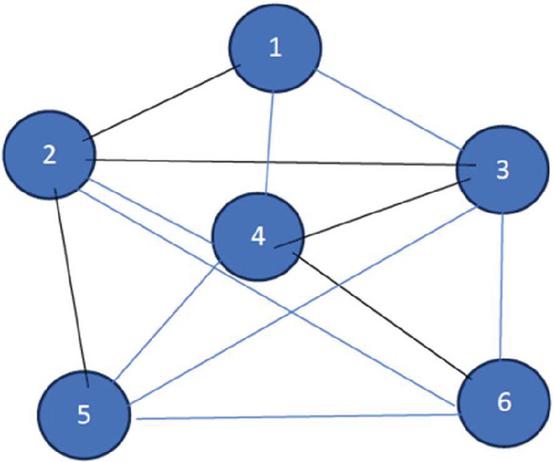
Let us reconsider the numerical illustration that was discussed in [1] and it was solved by the index restricted minimum connected graph approach. The network and link weights are given in Table 1, and Figure 1, respectively.
| F\T | 2 | 3 | 4 | 5 | 6 |
| 1 | 12 | 10 | 10 | – | – |
| 2 | – | 15 | 11 | 11 | 16 |
| 3 | – | 7 | 14 | 12 | |
| 4 | – | 10 | 11 | ||
| 5 | – | 9 |
Figure 1 Traveling salesman tour network.
Arranging the 13 link lengths from Table 1 in a non-decreasing order. This gives: 7(3,4), 9(5,6), 10(1,3), 10(1,4), 10(4,5), 11(2,4), 11(2,5), 11(4,6), 12(1,2), 12(3,6), 14(3,5), 15(2,3), 16(2,6).
Alternative 1: Note that links (3,4), (5,6), (1,3), can be selected. Link (1,4) forms a sub-cycle, hence not selected. Next selected link is (4,5), The next link that qualifies to be selected is the link (2,4), however, it will imbalance the index at node 4, which will become a high index node at index value of node 4 will be equal to 3. See Figure 2. Hence weights of links connecting node 4 are updated by quantity 1 and these new weights are shown in Table 2.
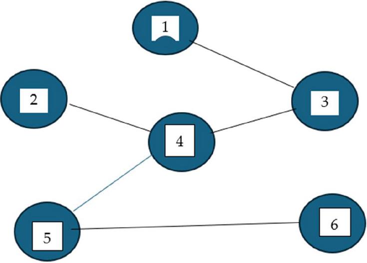
Figure 2 Nore 4 becomes imbalanced.
Table 2 Modified link weights for links emanating from node 4
| F\T | 2 | 3 | 4 | 5 | 6 |
| 1 | 12 | 10 | 10+1 | – | – |
| 2 | – | 15 | 11+1 | 11 | 16 |
| 3 | – | 7+1 | 14 | 12 | |
| 4 | – | 10+1 | 11+1 | ||
| 5 | – | 9 |
Alternative 2: Note that after selection of the links (3,4), (5,6), the next link (1,4), can be selected. Link (1,3) forms a sub-cycle, hence not selected. Next selected link is (4,5), This link brings an index imbalance at node 4, hence it requires updating of all links emanating from the node 4. Increasing weights of all nodes emanating from node 4 will resolve the tie in favour of the alternative 1, as the link (1,4) will have weight 11 compared to weight of the link (1,3) which will remain 10.
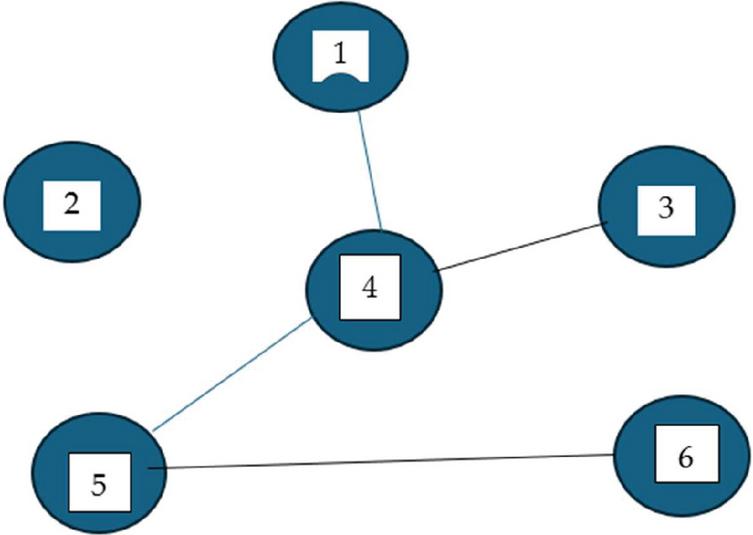
Figure 3 Alternative 2 at iteration 1.
Rearranging the link weights in increasing order, we have: 8(3,4), 9(5,6), 10(1,3), 11(1,4), 11(2,5), 11(4,5), 12(1,2), 12(2,4), 12(3,6), 12(4,6), 14(3,5), 15(2,3), 16(2,6).
Selected links will be 8(3,4), 9(5,6), 10(1,3). The next link (1,4) will not be included as it makes a cycle, however, the link (2,5) is selected. The next link (4,5) will make the node 5 imbalanced. Link weights emanating from the node 5 need updating. These weights are shown in Table 3 and network is shown in Figure 4.
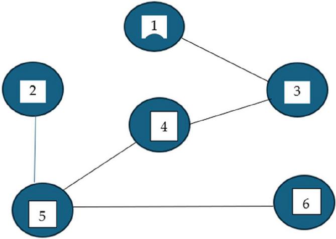
Figure 4 Selected links after updating link weights emanating from node 5.
These updated link-weights from Table 3 are rearranged in increasing order. 8(3,4), 10(1,3), 10(5,6), 11(1,4),), 12(1,2), 12(2,4), 12(2,5), 12(3,6), 12(4,5), 12(4,6), 15(2,3), 15(3,5), 16(2,6).
Table 3 Link weights after updating link weights emanating from node 5
| F\T | 2 | 3 | 4 | 5 | 6 |
| 1 | 12 | 10 | 11 | – | – |
| 2 | – | 15 | 12 | 11+1 | 16 |
| 3 | – | 8 | 14+1 | 12 | |
| 4 | – | 11+1 | 12 | ||
| 5 | – | 9+1 |
These link lengths will lead to the selection of the following: 8(3,4), 10(1,3), 10(5,6), 12(1,2), {12(2,4) not selected}, 12(2,5), 12(4,6). This is shown in Figure 5, which is the required travelling salesman tour. The cost associated with this tour can be obtained from Table 1, where the given cost data information prevails.
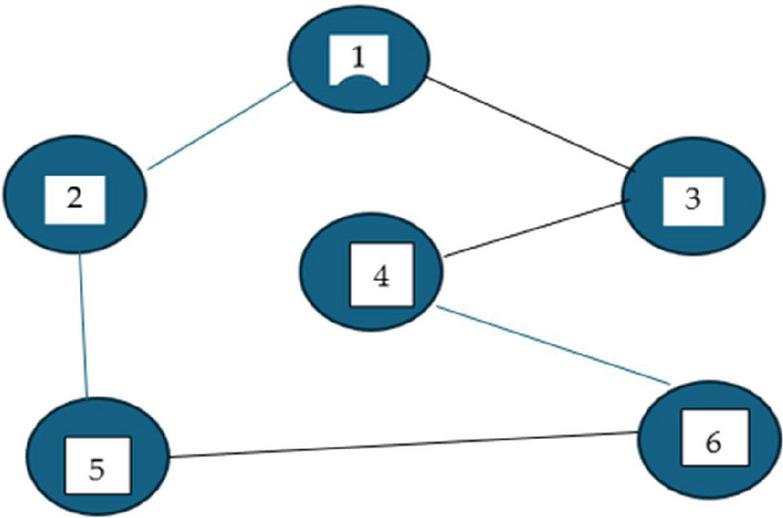
Figure 5 The required travelling salesman tour.
The cost of the travelling salesman tour will be given by 10 (1,3) +7 (3,4) +11 (4,6) +9 (6,5) +12 (5,2) +11 (2,1) = 60. It is an optimal solution as it is the same result as was obtained in [1]. However, it is desirable to establish its optimality independently from the available information.
It may also be noted that in the above example, sum of 6 minimum links turn out to be: 10 + 10 + 7 + 10 + 9 + 11 = 57. Therefore, the maximum error in the solution obtained above is = 3, or it is less than 6%, even if optimality of the above solution is disputed.
Note that the selection of the last link does not have any choice but only one possibility remains to make the tour feasible for the travelling salesman tour. In the above example, it was the link (4,6). From each node of the last link, at least two links will be included in the salesman tour. Let us look at the minimum links from the node 4 and the links from the node 6. These are:
Links from the node 4: 10(1,4), 11(2,4), 7(3,4), 10(4,5), and 11(4,6)
Links from the node 6: 16(2,6), 12(3,6), 11(4,6), and 9(5,6)
The salesman tour obtained from Figure 4 is comprised of the links 10(1,3), 7(3,4), 11(4,6), 9(6,5), 11(5,2), 12(2,1).
It may be noted that the minimum links from the node 4 and from the node 6 have been included in the salesman tour obtained by the proposed approach, However, the second minimum from the node 4 is not included but the included link is second minimum from the node 6 (in red) hence the solution obtained must be close to an optimal solution.
However, it remains a challenge to establish optimality of a solution for the travelling salesman problem obtained by the above heuristic. Here is one more attempt for resolving optimality of the solution by solving a slightly modified but equivalent data as given in Table 4. Since adding a constant does not change their relative merits of various values, we change the minimum link weight by adding a constant 3 to all links emanating from the node 3. This is given in Table 4.
Table 4 Slightly modified values of various link weights
| F\T | 2 | 3 | 4 | 5 | 6 |
| 1 | 12 | 10+3 | 10 | – | – |
| 2 | – | 15+3 | 11 | 11 | 16 |
| 3 | – | 7+3 | 14+3 | 12+3 | |
| 4 | – | 10 | 11 | ||
| 5 | – | 9 |
These link weights from Table 4 are rearranged in non-decreasing order as given below: 9(5,6), 10(1,4), 10(3,4), 10(4,5), 11(2,4), 11(2,5), 11(4,6), 12(1,2), 13(1,3), 15(3,6), 16(2,6), 17(3,5), 18(2,3). This results in the selection of 9(5,6), 10(1,4), 10(3,4), 10(4,5), which makes the node index of the node 4 more than 2. Hence, we add a constant to all links emanating from the node 4 as shown in Table 5.
Table 5 Modified values of link weights
| F\T | 2 | 3 | 4 | 5 | 6 |
| 1 | 12 | 13 | 10+1 | – | – |
| 2 | – | 18 | 11+1 | 11 | 16 |
| 3 | – | 10+1 | 17 | 15 | |
| 4 | – | 10+1 | 11+1 | ||
| 5 | – | 9 |
Arranging link weights from Table 5 in non-decreasing order, we have: 9(5,6), 11(1,4), 11(2,5), 11(3,4), 11(4,5), 12(1,2), 12(2,4), 12(4,6), 13(1,3), 15(3,6), 16(2,6), 17(3,5), 18(2,3). It will lead to the selection of 9(5,6), 11(1,4), 11(2,5), 11(3,4), and 11(4,5) resulting in high index of nodes 4 and 5, which give rise to Table 6.
Table 6 Modified values of link weights
| F\T | 2 | 3 | 4 | 5 | 6 |
| 1 | 12 | 13 | 11+2 | – | – |
| 2 | – | 18 | 12+2 | 11+1 | 16 |
| 3 | – | 11+2 | 17+1 | 15 | |
| 4 | – | 11+1+2 | 12+2 | ||
| 5 | – | 9+1 |
This results in the rearrangement of link-weights in non-decreasing order as. 10(5,6), 12(1,2), 12(2,5), 13(1,3), 13(1,4), 13(3,4), 14(2,4), 14(4,5), 14(4,6), 15(3,6), 16(2,6),) 18(2,3), 18(3,5). It will lead to:
(1) the selection of 10(5,6), 12(1,2), 12(2,5), 13(1,3), 13(3,4) and 14(4,6)
(2) rejection of 13(1,4), 14(2,4), 14(4,5).
The above is the same result as was shown in Figure 5.
Consider a completely connected 6-node, 15-link network taken from [16]. Its 15 link-weights are given Table 7. Network configurations are like the illustration 1.
Table 7 Link weights of the network
| nodes | 1 | 2 | 3 | 4 | 5 | 6 |
| 1 | – | 11 | 9 | 9 | 15 | 16 |
| 2 | 11 | – | 14 | 10 | 10 | 15 |
| 3 | 9 | 14 | – | 6 | 13 | 11 |
| 4 | 9 | 10 | 6 | – | 9 | 10 |
| 5 | 15 | 10 | 13 | 9 | – | 8 |
| 6 | 16 | 15 | 11 | 10 | 8 | – |

Figure 6 Reflecting selected links making node 4 a high index node.
Iteration 1: Arranging 15 link-weights in non-decreasing order as was done earlier in illustration 1, we have: 6(3,4), 8(5,6), 9(1,3), 9(1,4), 9(4,5), 10(2,4), 10(2,5), 10(4,6), 11(1,2), 11(3,6), 13(3,5), 14(2,3), 15(1,5), 15(2,6), 16(1,6).
The above weights will result in the selection of 6(3,4), 8(5,6), 9(1,3); rejection of 9(1,4), selection of 9(4,5) and 10(2,4); resulting in the index value 3 for the node 4. See Figure 6, link weights emanating from node 4 will need updating.
Iteration 2: Changing link-weights of links emanating from the node 4, we have:
{(6+1)(3,4)}, 8(5,6), 9(1,3), {(9+1)(1,4)}, {(9+1)}(4,5), {(10+1)(2,4)}, 10(2,5), {(10+1)(4,6)}, 11(1,2), 11(3,6), 13(3,5), 14(2,3), 15(1,5), 15(2,6), 16(1,6).
Rearranging in a non-decreasing order, we have:
7(3,4), 8(5,6), 9(1,3), 10(1,4), 10(2,5), 10(4,5), 11(1,2), 11(2,4), 11(3,6), 11(4,6), 13(3,5), 14(2,3), 15(1,5), 15(2,6), 16(1,6).
It will result in the selection of 7(3,4), 8(5,6), 9(1,3). The link 10(1,4) will be rejected and the link 10(2,5) and 10(4,5) will be selected. However, it will make node 5 a high index node, hence link-weights emanating from the node 5 need updating. See Figure 7.
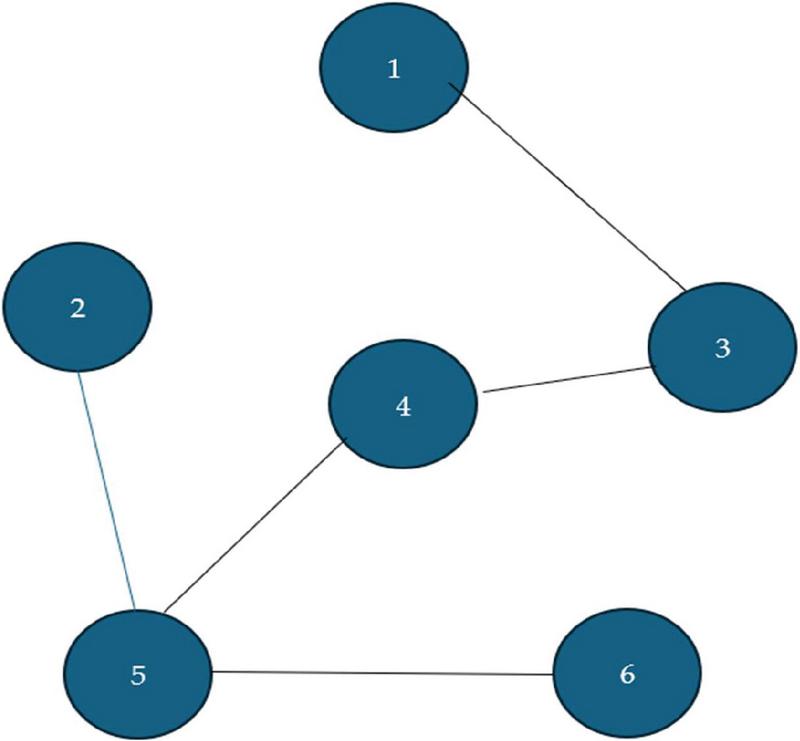
Figure 7 Network with high index node 5.
Iteration 3: The updated link weights will be:
7(3,4), {(8+1)(5,6)}, 9(1,3), 10(1,4), {(10+1)(2,5)}, {(10+1)(4,5)}, 11(1,2), 11(2,4), 11(3,6), 11(4,6), {(13+1)(3,5)}, 14(2,3), {(15+1)(1,5)}, 15(2,6), 16(1,6).
Rearranging these weights in a non-decreasing order, we have:
7(3,4), 9(5,6), 9(1,3), 10(1,4), 11(1,2), 11(2,4), 11(2,5), 11(3,6), 11(4,5)}, 11(4,6), 14(2,3), 14(3,5)}, 15(2,6), 16(1,5)}, 16(1,6).
This will lead to the selection of 7(3,4), 9(5,6), 9(1,3), rejection of 10(1,4), selection of 11(1,2), rejection of 11(2,4) and selection of 11(2,5); rejection of 11(3,6) and selection of 11(4,6). Once again, it is the same result that was obtained in [16].
This is an optimal solution to the salesman tour and is the same as was obtained earlier, shown in Figure 9. However, independent optimality of the solution needs further work.
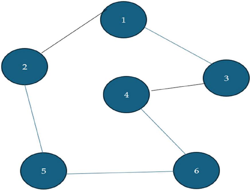
Figure 8 The minimum travelling salesman tour.
The above heuristic has provided optimal salesman tours; however, we could not establish optimality of a solution independently. In the next section, we follow strategy 3 discussed earlier in the Section 2.4, which results in an optimal solution.
Here, we develop a heuristic for identification of an index restricted shortest connected network joining the nodes p and p, which is a path between the nodes p and p, passing through all the remaining nodes of the given network. This path has an alternative interpretation, it also represents the travelling salesman tour, when nodes p and p are super imposed. This index restricted shortest connected network of the network , becomes the minimum travelling salesman tour for the network . The method gives an optimal salesman tour. Details can be seen in [5]. The steps for this modified approach are as follows:
Step 1. Given the network , identify a node with minimum number of links emanating from it. This requirement is not an essential requirement, as the required tour must pass through all nodes, therefore any node can be selected as the node p, from where the tour commences and finishes. For example, in the case of a completely connected network, the number of links emanating from all nodes will be equal, and we can select any node arbitrarily as the node p. The node .
Step 2. Given the network , reconstruct a network , i.e., duplicate of the node p is an extra node and all links emanating from the node p are also extra number of the links. Call the duplicate of the node p as p’ and all duplicate of all links (p, q) become (p, q). Since both link (p, q) and (p, q) cannot be selected as a member of the shortest connected network, hence once a link is selected for inclusion in the shortest connected network, its duplicate is set to . Note all other links have no duplicate links. Network links in are divided into two categories; links that do not change in their link-weights, are called Type 1 links, which includes all links other than those emanating from the node p, and Type 2 links are all links emanating from the node p and p. It is for this reason, the number of nodes in the reconstructed network are (N 1) and number of links are (.
Step 3: Create a counter K, and a set of selected links with initial values Note that in a n node network, the travelling salesman tour will have n number of links, which also forms a path between nodes p and p passing through all the remaining nodes. Therefore, when K n, or the number of selected links in the set is equal to n, the process will stop. Arrange Type 1 and Type 2 links in non-decreasing order and select the minimum weight link and go to Step 4. Initially, all links in Type 2 category will have link weights of two links equal. This link weight will change as and when a link is selected for inclusion in the minimum spanning tree.
Step 4: Select the minimum weight link, if (1) it does not form a loop with the existing selected links, and (2) if its selection is not increasing the index of the node p or p 1, and for any other node the index is not 2. Set K K+1 and include the selected link as a member of the set , and (3) in the case of Type 2 links, all links have an alternative, hence selection is done in favour of the node p or p, which satisfy the index requirement.
Step 5: If K n and , and if the selected link is of Type 1, return to Step 4. If the selected link is of Type 2, set the length of the duplicate equal to infinity. Re arrange links in non-decreasing order and return to Step 4. When K n, and , go to Step 6.
Step 6: Find the index restricted minimum spanning tree joining the nodes p and p and convert the spanning tree into the travelling salesman tour by superimposing nodes p and p, which is the required minimum salesman tour.
Let us reconsider the illustration 1 by the approach discussed in this section 5. The link weight for 13 links from Table 1 is reproduced as Table 8.
| F\T | 2 | 3 | 4 | 5 | 6 |
| 1 | 12 | 10 | 10 | – | – |
| 2 | – | 15 | 11 | 11 | 16 |
| 3 | – | 7 | 14 | 12 | |
| 4 | – | 10 | 11 | ||
| 5 | – | 9 |
From the Table 8, we note that the minimum number of links are emanating from the node 1. Hence this node is duplicated as node 1. Modified link-weights are given in Table 9.
Table 9 Link weights of the reconstructed network
| F\T | 1 | 1 | 2 | 3 | 4 | 5 | 6 |
| 1 | – | – | 12 | 10 | 10 | – | – |
| 1 | – | – | 12 | 10 | 10 | – | – |
| 2 | 12 | 12 | – | 15 | 11 | 11 | 16 |
| 3 | 10 | 10 | 15 | – | 7 | 14 | 12 |
| 4 | 10 | 10 | 11 | 7 | – | 10 | 11 |
| 5 | – | – | 11 | 14 | 10 | – | 9 |
| 6 | – | – | 16 | 12 | 11 | 9 | – |
From the above Table 9, we note that Type 1 links are 10 in number and Type 2 links are 6. Arranging these links in non-decreasing order, we have: Min {Type 1: {7(3,4), 9(5,6), 10(4,5), 11(2,4), 11(2,5), 11(4,6), 12(3,6), 14(3,5), 15(2,3), 16(2,6)}; Type 2: {10(1,3), 10(13), 10(1,4), 10(1,4), 12(1,2), 12(1,2)}}
One can easily see that minimum link- weights are: 7(3,4) and 9(5,6), which are selected, as they satisfy conditions stated in Step 4. Next minimum is 10(1,3), 10(1,3), 10(1,4), 10(1,4) and 10 (4,5). Note as was argued earlier, when the link 10(1,3) is selected, the corresponding duplicate link (1,3) is set equal to infinity, and length of the link (1,4) and (1,4) will be raised to 11 units as was explained in Illustration 1. Next minimum is link (4,5), which will increase the index of the node 4 to 3. Hence link-weights from node 4 needs updating.
| F\T | 1 | 1 | 2 | 3 | 4 | 5 | 6 |
| 1 | – | – | 12 | 10 | 10+1 | – | – |
| 1 | – | – | 12 | 10 | 10+1 | – | – |
| 2 | 12 | 12 | – | 15 | 11+1 | 11 | 16 |
| 3 | 10 | 10 | 15 | – | 7+1 | 14 | 12 |
| 4 | 10 | 10 | 11 | 7 | – | 10+1 | 11+1 |
| 5 | – | – | 11 | 14 | 10 | – | 9 |
| 6 | – | – | 16 | 12 | 11 | 9 | – |
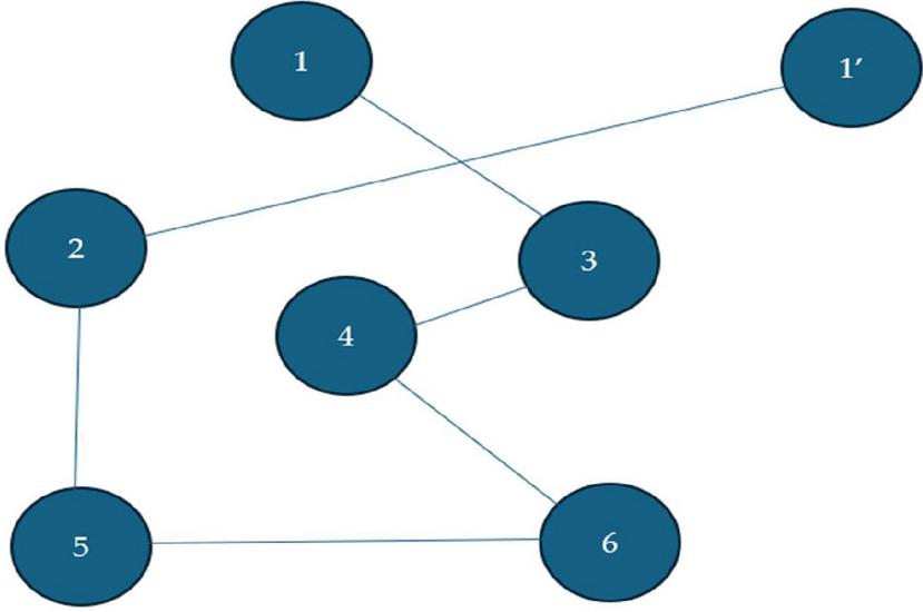
Figure 9 Reconstructed network.
{Type 1: {(7+1)(3,4), 9(5,6), (10+1)(4,5), (11+1)(2,4), 11(2,5), (11+1)(4,6), 12(3,6), 14(3,5), 15(2,3), 16(2,6)}, Type 2: {10(1,3), 10(13), (10+1)(1,4), (10+1)(1,4), 12(1,2), 12(1,2)}}
Following the steps, the selected links will be: (3,4), (5,6), (1,3), (2,5), (4,6), (1,2), which forms a IRMCN path joining the nodes 1 and 1 as shown in Figure 9. When nodes 1 and 1 are superimposed as one node, it forms the required minimum salesman tour as was shown in Figure 8.
In this paper, the index balancing theorem from [11] has been incorporated in the nearest neighbour heuristic [15] and link weights are reconstructed for an application of the greedy approach for the link selection.
The heuristic has been applied to some previously solved travelling salesman problem and this heuristic has identified optimal solutions; however, it is desirable to establish either some optimization conditions to check optimality of the solution obtained by the proposed heuristic approach or develop some independent proof for optimality of the solution given by the heuristic. This remains as a future work.
It is also desirable to establish some estimation for the maximum error in the solution obtained by the heuristic.
We have also established that instead of dealing with the given network, it may be desirable to deal with a reconstructed network, which is slightly larger than the given network, however, advantage is that it results in an optimal solution. Here we find the index restricted path between the node p and its duplicate node p’ and use its alternative interpretation to find the minimum travelling salesman tour, which is an optimal salesman tour. This discussion was presented in section 5, along with a numerical illustration.
In recent publications in [3–5] the authors have established optimality by considering various possibilities under different strategies. More computational work is needed to estimate computational advantage of this approach, and it will be reported in subsequent publications.
Once again, the question about the travelling salesman problem in the NP Hard category remains under dispute.
[1] Kumar, S. Munapo, E. (2024), Innovative ways of developing and using specific purpose alternatives for solving hard combinatorial network routing problems and ordered optimization problems, AppliedMath 2024, 4, 791–805, https://doi.org/10.3390/appliedmath4020042.
[2] Nemhauser, G., and Wolsey, L.A. (1988) Integer and combinatorial optimization, DOI: 10.1002/9781118627372, John Wiley & Sons, In.
[3] Kumar, S., Munapo, E., Lesaoana, M., and Nyamugure, P. (2017) Is the travelling salesman problem actually NP Hard? Chapter 3 in Engineering and Technology: Recent Innovations and Research, Editor Ashok Mathani, International Research Publication House, ISBN 978-93-86138-06-4, pp. 37–58.
[4] Kumar, S., Munapo, E., Lesaoana, M., and Nyamugure, P. (2018) A minimum spanning tree based approach to the travelling salesman problem, Opsearch, Vol. 55, No. 1, pp. 150–164, http://Doi10.1007/s12597-017-0318-5pp1-15.2017.
[5] Kumar, S., Munapo, E., Siguake, C., Al-Rabeeah, M. (2020a) The minimum spanning tree with node index =2 is equivalent to the minimum travelling salesman tour, Chapter 8, Mathematics in Engineering Sciences: Novel theories, Technologies and Applications, Ed Mangey Ram, Mathematical Engineering, Manufacturing, and Management Sciences Series, CRC Press https://www.crcpress.com/Mathematical-Engineering-Manufacturing-and-Management-Sciences/book-series/CRCMEMMS.
[6] Korte, B., and Vygen, J. (2006) Combinatorial optimization: Theory and Applications, Chapter 21, pp. 501–535, Springer.
[7] Christofides N. (2022) Worst-case analysis of a new heuristic for solving the travelling salesman problem, Operations Research Forum, 3:20, https://doi.org/10.1007/s43069-021-00101-z.
[8] Anupam, G. (2015) Deterministic MST, Advanced Algorithms, CMU, Spring 15-859E, pp. 1–6.
[9] Garg, R.C. and Kumar, S. (1968) Shortest connected graph through Dynamic Programming, Maths Magazine, Vol. 41, No. 4, pp. 170–173.
[10] Kruskal, J. B. (1956). On the shortest spanning subtree of a graph and the traveling salesman problem. Proceedings of the American Mathematical Society, 7(1), 48–50.
[11] Munapo, E., Kumar, S., Lesaoana, M., and Nyamugure, P. (2016) A minimum spanning tree with index =2, ASOR Bulletin, Volume 34, Issue 1, pp. 1–14.
[12] Munapo, E., Kumar, S, (2022) Linear Integer Programming: Theory, Applications and Recent Developments, Vol. 9, De Gruyter Series on the Applications of Mathematics in Engineering and Information Sciences, ISBN 978-3-11-070292-7.
[13] Munapo, E., Kumar, S, Nyamugure, P. and Tawanda, T. (2025) An Introduction to Network optimization by reconstruction, To be published by River’s publishers.
[14] Wikipedia, the free encyclopedia 10 Jan 2025.
[15] Yenigün, O (16 May 2023), Traveling Salesman Problem: Nearest Neighbor Algorithm Solution TSP in Python, Downloaded on 8 Jan 2025. Published in Dev Genious.
[16] Tawanda, T., Nyamugure, P., Kumar, S., and Munapo, E. (2023) A labelling method for the travelling salesman problem, Appl Sci. 2023, 13, 6417. httpa://doi.org/10.3390/app13116417.
[17] Kumar, S., Luhandjula, MK., Munapo, E., and Jones, B.C. (2010) Fifty years of Integer programming: A review of solution approaches, Asia Pacific Business Review, 6(2), pp. 5–15.
[18] Kumar, S., Munapo, E., Nyamugure, P., and Tawanda, T. (2022) Mathematics of OR: Significance of virtual directions in reducing computational complexity in network optimization, Chapter 3, Engineering trends in Applied research, Vol 3, Editor IS Chauhan, pp. 33–47, Integrated publication, New Delhi.
[19] Kumar, S., Munapo, E., Nyamugure, P., and Tawanda, T. (2024) Path through K specified nodes and links in a network, Journal of Graphic Era University, Vol. 12.2, pp. 263–282, doi: 10.13052/jgeu0975-1416.1225@ 2024 River Publishers.

Santosh Kumar OAM received PhD degree in Operations Research from Delhi University. He is author and co-author of over 220 papers and 4 books in Operations Research. His contributions in the field of OR were recognized by the Australian Society for Operations Research (ASOR)in 2009 by their ‘Ren Pots’ award. He has received a recognition award in 2011 for contributions in OR in Southern African region from the South African OR Society as a non-member of the society and a non-resident of South Africa. He was the President of the Asia Pacific Operations Research societies (1995–97), where ASOR was a member along with 7 other countries in the region. He is currently an Honorary Professor at RMIT University, Melbourne. He is a Chartered Mathematician and a Fellow of the Institute of Mathematics and its Applications, UK. On 14th June 2021, he was awarded under the Australian award system a medal of the Order of Australia (OAM).

Elias Munapo holds a BSc. (Hons) Applied Mathematics (1997), MSc. Operations Research (2002) and a PhD Operations Research (2010), all from the National University of science and Technology (N.U.S.T.), Zimbabwe. A certificate in outcomes-based assessment in Higher Education and Open distance learning, University of South Africa (UNISA), certificate in University Education Induction Program, University of KwaZulu-Natal (UKZN). He is a Professional Natural Scientist certified by the South African Council for Natural Scientific Professions (SACNASP), 2012; and NRF rated in South Africa. He has published/co-published over 140 articles and two books. He has also edited/co-edited 7 books and is a guest editor of Applied Sciences, Algorithms and Next Energy journals which are under MDPI. He has supervised/co-supervised eleven doctoral students and over 30 students at Master level. He is a member of the Operations Research Society of South Africa, Executive Committee Member 2012–13, South African Council for Natural Scientific Professions (SACNASP) as a Certified Natural Scientist, European Conference on Operational Research (EURO) and the International Federation of Operations Research Societies (IFORS), and a member of the International Conference on Optimization (ICO) and is part of the team preparing to host ICO 2026 at Johannesburg.
Journal of Graphic Era University, Vol. 13_2, 221–244.
doi: 10.13052/jgeu0975-1416.1321
© 2025 River Publishers