Data-Driven Retail Excellence: Machine Learning for Demand Forecasting and Price Optimization
Vinit Taparia, Piyush Mishra, Nitik Gupta and Hitesh Chandiramani*
Department of Mechanical Engineering, Malaviya National Institute of Technology Jaipur, Jaipur, Rajasthan, India
E-mail: tapariavinit1871@gmail.com; piyushmishra4112@gmail.com; 2019ume1662@mnit.ac.in; hiteshc2809@gmail.com
*Corresponding Author
Received 27 July 2023; Accepted 30 October 2023; Publication 21 November 2023
Abstract
Demand forecasting and price optimization are critical aspects of profitability for retailers in a supply chain. Retailers need to adopt innovative strategies to optimize pricing and increase profitability. This research paper proposes a price optimization approach for retailers using machine learning. The approach involves using linear regression to forecast demand incorporating price as an input, followed by price optimization taking into account inventory and perishability costs. The feasibility of using linear regression for price optimization for Stock Keeping Units (SKUs) is assessed using a feasibility index. The linear regression can predict the demand more accurately (23% Mean Absoulute Percentage Error (MAPE)) compared to exponential smoothing with optimised smoothing constant (47.09% MAPE) for 1000 SKUs. Also, the feasibility index can segregate the SKUs with an accuracy of 99%. The machine learning-based demand forecasting can assist retailers in accurately predicting customer demand and improving pricing decisions, while the feasibility index enables retailers to identify SKUs that require alternative pricing strategies.
Keywords: Demand forecasting, price optimization, inventory, linear regression, price elasticity, feasibility index.
1 Introduction
In a supply chain, the retailer is an important component as it acts as a link between the manufacturer and the customers, enabling the flow of goods. Retailers are at the forefront of supply chain responsiveness [1]. They play a vital role in minimizing stockouts, reducing lead times, and increasing product variety. There are majorly two kinds of retailing i.e., through offline retail outlets and through e-commerce platforms. Although, offline retailing dominates the market share but as noted by [2], there has been a proliferation in the use of e-commerce for shopping which has boosted post COVID-19. The percentage of offline retailing is steadily declining as more consumers turn to online shopping for convenience, discounts and high variety [3]. Offline retail stores can offer limited variety to the customers. However, accurate demand forecasting can assist the retailer in increasing the variety of products. This can be achieved if the retailer has the historical sales and price data. Incorporating price as an input in demand forecasting results in optimal outcomes as it impacts the overall demand for the product in the market [4]. The information can also help to maximise profit and optimise revenue under inventory and perishability constraints [3].
The offline retail industry is a highly competitive environment where retailers have to constantly devise ways of sustainability and growth [5]. One aspect of this is pricing each product correctly which is a crucial component of profitability [6]. It is a data-driven method that balances consumer demand and profitability of each sold item to maximize overall profits. Price optimization is constrained by inventory cost of outdated items and perishability cost. A surplus inventory of outdated items causes the shortage of inventory of other products [3]. Some items are perishable because of deterioration in value, technological changes and shift in consumer preferences [7]. Hence, for a perishable product supply chain, it is important to consider inventory control and determination of pricing.
This paper aims at proposing a price optimization approach making use of demand forecasting using machine learning. For this purpose, linear regression algorithm was used incorporating price as one of the inputs. We have used the linear regression algorithm because of its simplicity and easy interpretability by the retailer. Followed by demand prediction was the price optimization incorporating inventory and perishability costs. However, this technique has a drawback that we cannot use price optimization by linear regression for some SKUs, the identification of which can be done by using a feasibility index as described in the later sections.
The rest of the paper is organized as follows. Section 2 provides an overview of the literature on demand forecasting and price optimization. Section 3 describes the methodology used for the development of the price optimization approach and feasibility index. In Section 4, we present our numerical evaluation, results, and in Section 5 we discuss the implications of our findings.
2 Research Background and Literature Review
Accurate demand forecasting is essential for retaining a competitive edge along the supply chain in today’s changing industry. Improved demand forecasting enables consistent operations with reduced inventory costs across the whole supply chain [8]. Demand forecasting is estimating future demand for a good or service, which is influenced by a number of variables. By accurately estimating future consumer demands, retailers may make the best possible decisions regarding their purchases, inventory levels, production schedules, and resource allocation [8]. It is essential to include price as a variable in demand forecasting models since consumers frequently evaluate prices across stores when making purchasing decisions [9]. Additionally, fluctuations in the costs of related commodities might affect a product’s demand [10]. As a result, while projecting demand, we must take into account both our pricing strategy and market-competitive commodity prices to make wise pricing selections.
Price-demand interdependency has been studied in [11] in the domain of online fashion apparel retailing. The idea of price elasticity of demand, which gauges how responsive demand is to price fluctuations, is also covered. Moreover, demand will be extremely responsive to price changes if its price elasticity is high, which means that even tiny price fluctuations can have a big effect on demand. Markdown pricing is typical in fashion retailing because merchants strive to sell all of their inventory before the end of very short product life cycles, hence [12] implemented a markdown multi-product price decision support tool for fast-fashion retailer Zara.
A relationship between a dependent (predictor) variable and an independent (response) variable can be found using the statistical technique of linear regression. The goal is to determine whether or not the response variables can accurately predict the outcome variable [13]. Our research shows that one of the most useful things you can do with linear regression is to use the results to calculate the regression coefficients and the regression constant, which will allow you to create a simple mathematical function between the variables. [14] used Linear Regression (LR) and Least Squares Support Vector Machine – Artificial Bee Colony optimization (LSSVM-ABC), to predict product pricing in the market using previous prices. [15] addresses the dynamic pricing problem in case of unknown demand-price relation by proposing an approach that strikes the balance between revenue maximization and demand forecasting, by producing less myopic and profitable prices. [16] analyses prescriptive price optimisation, a technique that employs demand forecasting models for several items to determine the ideal pricing strategy that maximises future revenue or profit. They obtained several product demand forecasting models using parametric linear regression with feature modifications. The revenue maximisation problem was then recast as a binary quadratic optimisation (BQO) problem using the regression models, and techniques for effectively solving this problem were suggested. Econometrics modelling and multiple linear regression are used to optimize revenue for domestic flights by constructing market demand functions, discussing elasticity, cost degradation, and passenger diversion in [17]. [18] uses multiple regression, linear and nonlinear programming to propose a product-mix pricing method, applied to a sample of cleaning products in a retail store to analyse costs, model product relationships, and optimize prices for maximum profit.
Goods can be perishable due to physical deterioration, value deterioration, or shifts in consumer preferences and technological changes. Studying inventory control and pricing strategies becomes more crucial for a supply chain with perishable goods [4]. For a perishable commodity with unpredictable demand and no possibility of restocking, [19] created a pricing model. The challenge of pricing and ordering a perishable commodity with unpredictable price-sensitive demand is examined by [20]. The store determines product price and inventory allocation based on the prior period’s sales data, selecting the best pricing after determining the best order size, but assumes no inventory carryover. To estimate prices for a perishable commodity within a set time, [21] assumes negative binomial distribution of client demand and incorporates factors such as demand pace, buyer preferences, and sales period length for optimal pricing. [22] developed a model for a single product manufacturer facing continuous decay, price-dependent and time-varying demand, backlogged shortages, and multi-period planning horizon, aiming to optimize price and production lot-size/scheduling for maximum profit. Similarly, [23] analyzed pricing and inventory control for a perishable product with a fixed lifetime and first-in-first-out inventory consumption in an infinite horizon. [3] explores how past sales and pricing data can be utilized in offline retailing to optimize revenue under market and inventory constraints, by forecasting popular product demand, mitigating surplus inventory and losses from outdated products, optimizing prices to attract customers, and addressing seasonal demand trends, considering the limited stock and options available to customers and the increasing pressure to provide the best value for money. Using a dynamic pricing model to move through a fixed quantity of a perishable commodity in a finite amount of time, [24] demonstrate how to maximise profits by adopting dynamic optimum policies. The maximum profit function is also shown to be continuously piecewise concave by [25], who use a multiperiod inventory and pricing model for a single product at the retail end of the supply chain. However, a gap that exists in current literature streams is that there has not been any method proposed regarding the segregation of SKUs on the basis of their demand patterns and thereby impacting adoption of different pricing policies for these SKUs. This segregation of SKUs is an important factor that influences the decisions of managers and therefore the overall profitability of the retailers. In this paper, we have developed a feasibility index for this purpose about which we have described in the later section.
3 Methodology
This section comprises of a description of the methodology that has been adopted for demand prediction, price optimization and development of the feasibility index. The section has been divided into four subsections. Section 3.1 talks about the data and its pre-processing. Section 3.2 describes about input to the linear regression algorithm. Section 3.3 briefs about the methodology for demand prediction and price optimization and Section 3.4 elucidates the methodology to develop feasibility index.
3.1 Dataset and Pre-processing
The dataset contains the weekly demand and price data of 1000 SKUs for a retail store for 104 weeks. The demand data for most of the SKUs were found to be normally distributed. There were a few weeks when a sudden rise (more than 400%) in demand was observed. The sudden rise in demand is considered an outlier, and these outliers were replaced by random values near the average demand to improve the quality of the forecast.
Data were divided into four sets. 1–52 weeks for finding optimised smoothing constant, seasonality factor, and trend analysis; 53–94 weeks for training the linear regression algorithm and 95–104 for testing the algorithm.
3.2 Input for Linear Regression Algorithms
(a) To consider historical demand, we first predicted the demand from exponential smoothing with the optimised value of the smoothing constant for every SKU using an excel solver with multi-start as suggested by [26] using VBA. Then, the predicted demand is taken as one of the inputs for the regression algorithms. It helps us to focus on the recent variations in demand.
(b) A trendline was fit on training data, and a trend prediction was obtained for testing data. A seasonality factor was calculated, which measures that, on average, demand for a time interval is above or below normal. The trend prediction was multiplied by the seasonality factor to obtain the prediction from trend and seasonality analysis, which is the second input to our model. Trend analysis helps examine the overall direction or pattern in a demand over time. This can help identify long-term changes or patterns in the data, such as whether the demand is increasing, decreasing, or staying relatively stable. Seasonality analysis involves examining demand patterns that repeat themselves in a time series over shorter periods, such as daily, weekly, or monthly cycles.
(c) Price is taken as the third input for the regression algorithms.
3.3 Forecasting Methodology
This data was the used in the linear regression model for prediction. Through linear regression we got the regression constants and the equation. This way, one can have the function which can be used to predict the demand using different values of price. Notably, the prediction from trend and seasonality analysis and exponential smoothing would be considered as constants for this estimate because they are made using the historical data and only price is variable. The output of the demand prediction thus, serves as an input to the price optimization methodology the flow diagram of which has been shown in Figure 1.
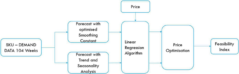
Figure 1 Methodology for price optimization.
The demand function thus obtained using linear regression was
| (1) |
Where,
D Demand
P Price
The corresponding profit function was then written as:
| (2) |
The optimum value of price for which the profit is maximum was determined by differentiating Equation (2). However, if the predicted demand at the optimum value of price comes out to be less than the inventory in hand (I), the profit function must account for the inventory and perishability cost.
The profit function when is:
| (3) |
Where, C Inventory cost
S.T :
| (4a) | ||||
| (4b) | ||||
Where
Perishability index associated with the SKU
Average price of SKU
3.4 Methodology for the Feasibility Index
It is a notable feature that not for all the SKUs, demand will vary with the price i.e., the price elasticity of demand is fairly low which is usually observed in goods that are essential having fewer substitutes [27]. Moreover, this can be validated from the analysis of regression coefficients thus obtained, where we found that for some SKUs the coefficient of price was very low which suggests that there might be some SKUs where fluctuations in price would not impact the demand significantly. In such cases, the value of optimum price lies beyond a certain rational range and therefore we cannot use our model. Since Customers know the best price for products, we need the optimized price should be in a particular range [3]. There were also some SKUs where the coefficient of price was less and still the value of optimum price fell beyond range suggesting that it is not the only criteria. Thus, before carrying out price optimization analysis, such SKUs must be identified and for this purpose, we have come up with an index called the feasibility index. The value of this index depends upon the price range of the SKU, average demand and coefficient of price. Table 1 gives inference of different values of . The formula of the feasibility index is as follows:
| (5) |
Table 1 Interpretation of different values of
| Sr. No. | Range of | Inference |
| 1 | Optimum price falls beyond range | |
| 2 | Optimum price is near the range | |
| 3 | Optimum price falls within the range |
4 Results
The forecast generated from exponential smoothing with optimised alpha was compared with that generated using linear regression. The results showed that the average MAPE for linear regression (23%) was lesser as compared to that of exponential smoothing (47.09 %) for 1000 SKUs. This shows that demand prediction using linear regression is a better and a more accurate approach. Moreover, the validity of the feasibility index was tested on these SKUs and it was found that the inference of held true for 98.79% of the cases, while that of held true for 98.89% of the cases.
5 Conclusion and Discussion
Demand forecasting and price optimization is crucial for the success of a retailer in a supply chain. Traditional methods of demand forecasting have been replaced by machine learning algorithms because of better accuracy. In this paper, we have used the linear regression algorithm because its easy to understand, simple to use and we can obtain the regression equation i.e., the demand function. We first generated a trend and seasonality analysis thereby incorporating the general trend as to how the demand is going to vary along with the seasonal factor considering the seasonal demand. This was followed by generating the prediction using exponential smoothing with optimized alpha for which we had used the solver available in excel ensuring the multistart option. Using excel solver integrated with the VBA tool in excel is an easy way to find optimized smoothing constant. This prediction was then compared with that generated by linear regression. Our findings validate that linear regression is a better model for prediction as compared to conventional methods such as exponential smoothing with optimized alpha. The price optimization model used the prediction from linear regression as an input and was solved under the inventory constraints. However, in our model, we have assumed continuous flow of inventory into the system and thus, the study can be further extended by incorporating the supply constraints. Also, a limitation of our literature is that it doesn’t provide any information about the pricing decision methodology for the SKUs for which the optimum price falls beyond range and thus, it can be extended further considering different pricing decisions. Furthermore, the identification of SKUs for which we cannot use the model due to fairly low-price elasticity was to be determined so that a different pricing policy can be used for such SKUs as the price obtained from our model would then be out of the consumer preference pricing range. Thus, we had developed a feasibility index which would help the mangers easily segregate the SKUs accordingly. The feasibility index was found out to be around 99% accurate when tested on the 1000 SKUs and thus, can be used by retailers with the availability of historical demand and price data. Hence, by identification of these SKUs, managers can make better decisions regarding pricing policies of different SKUs and accordingly manage inventory flow in and out of the system keeping in touch with the consumer demand.
References
[1] Sandberg, Erik & Jafari, Hamid. (2018). Retail supply chain responsiveness – Towards a retail-specific framework and a future research agenda. International Journal of Productivity and Performance Management. 67. 00–00. DOI: 10.1108/IJPPM-11-2017-0315. https://www.researchgate.net/publication/328391331\_Retail\_supply\_chain\_responsiveness\_-\_Towards\_a\_retail-specific\_framework\_and\_a\_future\_research\_agenda.
[2] Report on Retail Research, Accenture. https://www.accenture.com/\_acnmedia/PDF-130/Accenture-Retail-Research-POV-Wave-Seven.pdf.
[3] T. Qu, J.H. Zhang, Felix T.S. Chan, R.S. Srivastava, M.K. Tiwari, Woo-Yong Park, Demand prediction and price optimization for semi-luxury supermarket segment, Computers & Industrial Engineering, Volume 113, 2017, Pages 91–102, ISSN 0360-8352, https://doi.org/10.1016/j.cie.2017.09.004. (https://www.sciencedirect.com/science/article/pii/S0360835217304023).
[4] Gaurav Gupta – An analyses and evolution of Indian retail market in current scenario (A case study of some selected companies in India after Globalization).
[5] Lapinskaitë, Indrë and Kuckailytë, Justina. (2014). The Impact of Supply Chain Cost on the Price of the Final Product. Business, Management and Education. 12. 109–126. DOI: 10.3846/bme.2014.08. (https://www.researchgate.net/publication/272857284\_The\_Impact\_of\_Supply\_Chain\_Cost\_on\_the\_Price\_of\_the\_Final\_Product).
[6] Junxiu Jia, Qiying Hu, Dynamic ordering and pricing for a perishable goods supply chain, Computers & Industrial Engineering Volume 60, Issue 2, 2011, Pages 302–309, ISSN 0360-8352, https://doi.org/10.1016/j.cie.2010.11.013. (https://www.sciencedirect.com/science/article/pii/S0360835210003098).
[7] Kimitoshi Sato, Katsushige Sawaki, A continuous-time dynamic pricing model knowing the competitor’s pricing strategy, European Journal of Operational Research, Volume 229, Issue 1, 2013, Pages 223–229, ISSN 0377-2217, https://doi.org/10.1016/j.ejor.2013.02.022. (https://www.sciencedirect.com/science/article/pii/S0377221713001550).
[8] Sushil Punia, Konstantinos Nikolopoulos, Surya Prakash Singh, Jitendra K. Madaan and Konstantia Litsiou (2020) Deep learning with long short-term memory networks and random forests for demand forecasting in multi-channel retail, International Journal of Production Research, 58:16, 4964-4979, DOI: 10.1080/00207543.2020.1735666. https://www.tandfonline.com/doi/full/10.1080/00207543.2020.1735666.
[9] Kimitoshi Sato, Katsushige Sawaki, A continuous-time dynamic pricing model knowing the competitor’s pricing strategy, European Journal of Operational Research, Volume 229, Issue 1, 2013, Pages 223–229, ISSN 0377-2217, https://doi.org/10.1016/j.ejor.2013.02.022. (https://www.sciencedirect.com/science/article/pii/S0377221713001550).
[10] Sethuraman, R., Srinivasan, V., and Kim, D. (1999). Asymmetric and Neighborhood Cross-Price Effects: Some Empirical Generalizations. Marketing Science, 18(1), 23–41. http://www.jstor.org/stable/193249.
[11] Ferreira, Kris, Lee, Bin and Simchi-levi, David. (2015). Analytics for an Online Retailer: Demand Forecasting and Price Optimization. Manufacturing & Service Operations Management. 18. DOI: 10.1287/msom.2015.0561. https://www.researchgate.net/publication/283817399\_Analytics\_for\_an\_Online\_Retailer\_Demand\_Forecasting\_and\_Price\_Optimization.
[12] Felipe Caro, Jérémie Gallien – Clearance Pricing Optimization for a Fast-Fashion Retailer Vol. 60, No. 6, November–December 2012, pp. 1404–1422 ISSN 0030-364X http://dx.doi.org/10.1287/opre.1120.1102. http://personal.anderson.ucla.edu/felipe.caro/papers/pdf\_FC15.pdf.
[13] Yunus Kologlu, Hasan Birnici, Savde Ilgaz Kanalmaz, Burhan Oyzilmaz, “A Multiple Linear Regression Approach For Estimating the Market value of Football players in Forward position”.
[14] Mohamed Zaim Shahrel, Sofianita Mutalib and Shuzlina Abdul-Rahman- PriceCop – Price Monitor and Prediction Using Linear Regression and LSVM-ABC Methods for E-commerce Platform I.J. Information Engineering and Electronic Business, 2021, 1, 1–14 Published Online February 2021 in MECS (http://www.mecs-press.org/) DOI: 10.5815/ijieeb.2021.01.01.
[15] Dina Elreedy, Amir F. Atiya, and Samir I. Shaheen – Multi-Step Look-Ahead Optimization Methods for Dynamic Pricing with Demand Learning – Received April 28, 2021, accepted June 3, 2021, date of publication June 8, 2021, date of current version June 28, 2021. Digital Object Identifier 10.1109/ACCESS.2021.3087577. https://ieeexplore.ieee.org/stamp/stamp.jsp?arnumber=9448193\&tag=1.
[16] Shunnosuke Ikeda, Naoki Nishimura, Noriyoshi Sukegawa and Yuichi Takano – Prescriptive price optimization using optimal regression trees-Product Development Management Office, Recruit Co., Ltd., 1-9-2 Marunouchi, Chiyoda-ku, 100-6640, Tokyo, Japan. Faculty of Engineering, Information and Systems, University of Tsukuba, 1-1-1 Tennodai, Tsukuba-shi, 305-8573, Ibaraki, Japan. https://optimization-online.org/wp-content/uploads/2023/01/Prescriptive\_Price\_Optimization\_Using\_Optimal\_Regression\_Trees-1.pdf.
[17] Betty Rene´e Ferguson and Don Hong – Airline Revenue Optimization Problem: a Multiple Linear Regression Model, Journal of Concrete and Applicable Mathematics, Vol. 5, No.2, 153–167, 2007, Copyright 2007 Eudoxus 153 Press, LLC. https://www.mtsu.edu/faculty/dhong/publications/FergusonHong07.pdf.
[18] Jorge Eduardo Scarpin and Lara Fabiana Dallabona – Pricing and profit maximization: a study on multiple products. https://www.pomsmeetings.org/ConfProceedings/065/Full\%20Papers/Final\%20Full\%20Papers/065-1901.pdf.
[19] Gallego, Van Ryzin, (1994) Optimal Dynamic Pricing of Inventories with Stochastic Demand over Finite Horizons. Management Science 40(8):999–1020, https://doi.org/10.1287/mnsc.40.8.999. https://pubsonline.informs.org/doi/10.1287/mnsc.40.8.999.
[20] Apostolos N. Burnetas, Craig E. Smith, (2000) Adaptive Ordering and Pricing for Perishable Products. Operations Research 48(3):436–443. https://doi.org/10.1287/opre.48.3.436.12437. https://pubsonline.informs.org/doi/10.1287/opre.48.3.436.12437.
[21] Young H. Chun, Optimal pricing and ordering policies for perishable commodities, European Journal of Operational Research, Volume 144, Issue 1, 2003, Pages 68–82, ISSN 0377-2217, https://doi.org/10.1016/S0377-2217(01)00351-4. (https://www.sciencedirect.com/science/article/pii/S0377221701003514).
[22] Jen-Ming Chen, Liang-Tu Chen, Pricing and production lot-size/ scheduling with finite capacity for a deteriorating item over a finite horizon, Computers & Operations Research, Volume 32, Issue 11, 2005, Pages 2801–2819, ISSN 0305-0548, https://doi.org/10.1016/j.cor.2004.04.005. (https://www.sciencedirect.com/science/article/pii/S0305054804000796).
[23] Yanzhi Li, Andrew Lim, Brian Rodrigues, (2008) Note—Pricing and Inventory Control for a Perishable Product. Manufacturing & Service Operations Management 11(3):538–542. https://doi.org/10.1287/msom.1080.0238. https://pubsonline.informs.org/doi/10.1287/msom.1080.0238.
[24] Zhao, W., and Zheng, Y.-S. (2000). Optimal Dynamic Pricing for Perishable Assets with Nonhomogeneous Demand. Management Science, 46(3), 375–388. http://www.jstor.org/stable/2634737.
[25] S. Bhattacharjee and R. Ramesh, “Multi-period profit maximizing model for retail supply chain management: an integration of demand and supply-side mechanisms,” European Journal of Operational Research, vol. 122, no. 3, pp. 584–601, 2000. https://www.jstor.org/stable/2634737.
[26] Handanhal V. Ravinder. “Determining the optimal values of Exponential Smoothing Constants – Does Solver really work?”, American Journal of Business Education, vol. 6, no. 3.
[27] Patrick L. Anderson, Richard D. McLellan, Joseph P. Overton, and Dr. Gary L. Wolfram | Nov. 13, 1997 – Price Elasticity of Demand.
Biographies

Vinit Taparia did his B.Tech in Mechanical Engineering from Malaviya National Institute of Technology, Jaipur, Rajasthan. Currently he is working on Gas and Power Projects. His research interests include supply chain management, demand planning, inventory management, and renewable energy sources.

Piyush Mishra completed his B.Tech in Mechanical Engineering from Malaviya National Institute of Technology Jaipur, Rajasthan. He is currently employed in Reliance Industries in FCC unit of DTA Refinery. His research interests include supply chain management, demand planning, inventory management and planning.

Nitik Gupta completed his B.Tech in Mechanical engineering from Malaviya National Institute of Technology, Jaipur, Rajasthan. He is currently employed in Fernweh Group, a private equity firm as an Analyst focusing on Industrials sector and its sub-sectors. His research interests include supply chain management, demand planning & inventory management.

Hitesh Chandiramani completed his B.Tech in Mechanical engineering from Maharishi Arvind Institute of Engineering and Technology, Jaipur, Rajasthan. He completed his Master’s in Industrial Engineering and Management from UD, RTU, Kota. His research interests include Reliability Engineering, Operations Research, and Applied Statistics.
Journal of Graphic Era University, Vol. 12_1, 37–52.
doi: 10.13052/jgeu0975-1416.1213
© 2023 River Publishers