Improved Demand Forecasting of a Retail Store Using a Hybrid Machine Learning Model
Vinit Taparia, Piyush Mishra, Nitik Gupta and Devesh Kumar*
Department of Mechanical Engineering, Malaviya National Institute of Technology Jaipur, Jaipur, Rajasthan, India
E-mail: tapariavinit1871@gmail.com; piyushmishra4112@gmail.com; 2019ume1662@mnit.ac.in; deveshkumar1993@gmail.com
*Corresponding Author
Received 27 July 2023; Accepted 27 October 2023; Publication 21 November 2023
Abstract
Accurate demand forecasting is a competitive advantage for all supply chain components, including retailers. Approaches like naïve, moving average, weighted average, and exponential smoothing are commonly used to forecast demand. However, these simple approaches may lead to higher inventory and lost sales costs when the trend in demand is non-linear. Additionally, price strongly influences demand, and we can’t neglect the impact of price on demand. Similarly, the demand for a stock keeping unit (SKU) depends on the price of the competitor for the same SKU and the price of the competitive SKU. We thus propose a demand prediction model that considers historical demand data and the SKU price to forecast the demand. Our approach uses different machine-learning regressor algorithms and identifies the best machine-learning algorithm for the SKU with the lowest forecasting error. We further extend the forecasting model by training a hybrid model from the best two regression algorithms individually for each SKU. Forecasting error minimisation is the driving criterion for our literature. We evaluated the approach on 1000 SKUs, and the result showed that the Random Forest is the best-performing regressor algorithm with the lowest mean absolute percentage error (MAPE) of 8%. Furthermore, the hybrid model resulted in a lower inventory and lost sales cost with a MAPE of 7.74%. Overall, our proposed hybrid demand forecasting model can help retailers make informed decisions about inventory management, leading to improved operational efficiency and profitability.
Keywords: Demand forecasting, inventory optimisation, machine learning, hybrid model, price elasticity.
1 Introduction
In today’s dynamic market, accurate demand forecasting is crucial for maintaining a competitive edge in the supply chain. Better demand forecasts allow reliable operations at low inventory costs throughout the entire supply chain [1]. Demand forecasting involves predicting the future demand for a product or service, which is influenced by various factors. Accurate forecasting allows companies to optimize their purchase decision, inventory levels, production schedules, and resource allocation to meet future customer demands [2]. Despite its importance, demand forecasting remains a challenging task, especially when the trend in demand is non-linear [3]. Traditionally, companies have relied on simple statistical methods like naïve, moving averages, weighted averages, and exponential smoothing to forecast demand [4, 5]. Such easy-to-use techniques are valued for their simplicity; however, they may not be suitable for capturing the complexities of modern supply chains, where demand is influenced by various factors such as pricing, promotions, and competitor actions.
Neglecting to include price as an input in demand forecasting can result in suboptimal outcomes, as it can change the overall demand for the product in the market [6]. Additionally, consumers typically compare prices among different retailers when making purchase decisions, making it crucial to include price as a variable in demand forecasting models [7]. Furthermore, variations in prices of comparable commodities can also influence demand for a product [8]. Therefore, we must consider both our pricing strategy and competitive commodity prices when forecasting demand to make informed pricing decisions.
Researchers have turned to machine learning techniques to address these challenges to improve demand forecasting accuracy [9]. Machine learning algorithms can analyse large volumes of historical data, identify patterns and trends, and generate more accurate demand forecasts. Additionally, machine learning algorithms can incorporate various external factors like pricing, promotions, and competitor actions, making them ideal for modern supply chains.
This paper proposes a demand prediction model that leverages historical demand data and SKU pricing information to forecast demand accurately. Specifically, we evaluate the performance of five popular machine learning algorithms – Linear Regression, Polynomial Regression, Support Vector Regression, Decision Tree Regression, and Random Forest Regression – to identify the best-performing algorithms for forecasting demand for each SKU. We also develop a hybrid model that combines the two best-performing algorithms for each SKU to improve forecast accuracy further.
The rest of the paper is organized as follows. Section 2 provides an overview of the literature on demand forecasting and machine learning techniques. Section 3 describes the methodology used for developing and evaluating our demand prediction model. In Section 4, we present our numerical evaluation results, and in Section 5, we discuss the implications of our findings and highlight future research directions.
2 Research Background and Literature Review
Demand forecasting is one of the most essential components of supply chain management, directly influencing a company’s overall performance and competitiveness [10]. It is an important task for retailers as it is required for various operational decisions [11]. It goes without saying that if an organization does not get its forecasting accurate to a reasonable level, the whole supply chain gets affected [12]. Based on the paper’s objective, we focus on demand prediction techniques, specifically machine learning regression algorithms and hybrid models to forecast demand.
2.1 Demand Forecasting
Time series methods, including moving average, simple exponential smoothing, holt’s model, and Winter’s model, have been used to forecast the demand [13]. Research has been carried out to optimise these traditional methods such as [14] proposes the method to optimise exponential smoothing constant value using Excel Solver. The commonly used demand-forecasting methods such as Moving Average, Naïve Approach, or Exponential Smoothing are easily proposed to forecast trends in time-series data due to their simple and economic use, ease of understanding, and implementation. These approaches use previous demand data to predict the demand, focusing more on recent demand data. However, a criticism of this literature stream is that it doesn’t forecast accurately when the trends are non-linear and dependent on various factors. Compared with traditional statistical techniques, machine learning showed better sales forecasting, as demonstrated by higher accuracy than previous models, the flexibility to handle more data variables, and the capacity to process large data volumes [15]. [16] compared advanced machine learning techniques, including neural networks, recurrent neural networks, and support vector machines, to forecasting distorted demand with traditional methods, including naïve forecasting and moving averages. They concluded that using machine learning techniques to forecast distorted demand provides more accurate forecasts than simpler forecasting techniques (including naïve, trend, and moving averages). Therefore, many researchers have used machine learning to forecast demand. For example, [17] has used machine-learning algorithms, such as Linear Regression and Gradient Boosting Trees (an ensemble machine learning technique that combines multiple decision trees to make accurate predictions by iteratively focusing on the errors of previous trees) to predict the demand more accurately. They analysed previous years’ sales data and recorded its pattern to predict future trends. Similarly, [18] has used machine learning for hotel demand forecasting.
2.2 Machine Learning Algorithms
Forecasting techniques such as Autoregressive integrated moving average (ARIMA) which models future data points as a combination of past observations, their differences, and moving averages to make predictions dominated the forecasting field for many years. With the progression of time, the complexities of problems and the scope of datasets widened and posed various challenges for traditional methods. The machine learning discipline contains a lot of powerful methods and algorithms to handle complex datasets [19]. Machine learning refers to using and developing computer systems that can learn and adapt by using algorithms and models to analyse and draw inferences from patterns in datasets.
Various models for problems like regression, classification and clustering have been developed. Some of the models and algorithms to be used are described below:
Linear Regression: Linear Regression is a statistical tool that establishes a relationship between a dependent (predictor) variable and an independent (response) variable. The objective is to examine whether the response variables are able to predict the outcome variable successfully or not. One of the major applications of linear regression that we found is that it gives us the values of the regression coefficients and the regression constant, which would be helpful in establishing an easily interpretable mathematical function between the variables this function can then be used for the optimization techniques. [20] conducted multiple regression analyses to forecast the market value of football players at forward positions. Raghavan et al. [21] used linear regression analysis to predict the demand for housing space required due to the growing population in the Erode district of Tamil Nadu. Other studies have also utilized linear regression in various applications. For instance, [22] used multiple regression for forecasting the exchange rate using the aggregation operators considering inflation and interest rates as the inputs. [23] used both linear and multivariate adaptive regression spline models for the forecasting of evapotranspiration of the crop for effective vineyard irrigation management. A multiple linear regression model was used by [24] to estimate the project cost in a general project management field for earned value management. Additionally, a neural network and linear regression-based model was developed by [25] for the forecasting of photovoltaic power incorporating power generation, geographical and metrological data along with historical weather data. [26] created an advanced and integrated model using a genetic algorithm, Artificial Neural Network and linear regression models to predict energy demand. [27] used actual industrial data in Iran to develop a prediction model using linear regression for energy demand in the industries. A prediction-based model was proposed by [28] using regression, rule-based, and tree-based methods to predict spare parts demand in the bus fleet industry. Furthermore, linear regression, genetic algorithm, and LR-GA-based hybrid model were employed by [29] for accurately forecasting the demand in the private residential market. Lastly, [30] studied the combination of statistical and regression models for forecasting long-term and short-term demand in retail outlets, thereby considering both temporal and covariates-based variations. However, the accuracy of this technique depends on how linearly separated the data points are, and most of the real-life problems have outliers and some relationships between the independent variables as well, which tend to reduce the accuracy of this technique.
However, the accuracy of this technique depends on how linearly separated the data points are, and most of the real-life problems have outliers and some relationships between the independent variables as well, which tend to reduce the accuracy of this technique.
A simple linear regression is a model with a single independent variable x that has a relationship with a response y with a straight line. The model is expressed as:
| (1) |
where the intercept and the slope are unknown constants, and is a random error component.
However, if there is more than one regressor x (where the response variable may be related to regressors x1, x2, …, xi), then it is known as multiple linear regression, the model of which is expressed as:
| (2) |
Polynomial Regression: The assumption of the linear relationship between the features and response variable is not often the case in real-life scenarios. Polynomial regression is useful when the dataset has a curvilinear relationship [32]. The assumption of the linear relationship between the features and response variable is not often the case in real-life scenarios. Polynomial regression models have been used in various fields for demand forecasting, sales prediction, and tourism demand prediction. For example, [33] developed a cubic polynomial-based model for predicting international tourism arrivals in Singapore, while [34] used a polynomial regression model to develop a prediction model between sales and promotional prices. In addition, [35] used multiple linear regression and polynomial functions-based prediction models for demand forecasting in pharmaceutical supply chains. The polynomial regression algorithm has also been combined with other algorithms, such as random forest regression, to improve demand forecasting accuracy in the newsvendor problem [36]. The Polynomial is a form of linear regression in which the relationship between dependent and independent variables is modelled as nth degree polynomial in x. Mathematically, the polynomial regression equation can be expressed as:
| (3) |
Where
i are the slopes of the regression line
i are the weights of individual polynomial fit variables
0 is the intercept
n number of features in the dataset [37].
Decision Tree Regression: A decision tree is one of the most common and practical approaches for supervised learning that can be used to solve both classification and regression problems. The given data points are first plotted, and the models are then obtained by recursively partitioning the data space and fitting the data into simple prediction models at each partition [38]. Johnsons et al. used regression trees for demand prediction and price optimization for Rue La La, an online retailer [39]. Once the dataset is recursively split using a decision tree and is trained, a new data point (from test data) is passed through the root nodes and eventually comes at a leaf node where the prediction is obtained. The prediction is obtained by simply averaging out the values of all the trained data points in that leaf node. While splitting the nodes, the variance reduction of the data points at each node is calculated, and the splitting condition that gives the least variance is considered. This way, the model gets the best splitting conditions and is trained accordingly.
| (4a) | |||
| (4b) | |||
Support Vector Regression: Akin to linear regression, which requires a straight line to fit the data, this model incorporates a plane known as the hyperplane. Any SVM model has its objectives concerning the fitting and optimisation of a hyperplane in n-dimensional space to classify the data points strictly. Unlike other regression models, SVR tries to minimise the threshold value, i.e., the distance between the data point and the hyperplane. The “best-fit line”, i.e., the hyperplane, consists of the maximum number of points. For problems concerning low sample space and more features, SVR gives the best accuracy. Moreover, the computational complexity of this model doesn’t depend on the input space [40]. A support vector regression model was proposed by [41] for the demand forecasting of energy products such as coal, oil, natural gas and electricity. [42] proposed using SVR to predict product demand quantity in the computer, consumer electronics and communications market. [43] proposed an adaptive and flexible regression function using support vector regression analysis and linear and non-linear programming functions for identifying the underlying customer demand patterns using historical customer demand patterns. The results showed a prediction accuracy of more than 93%. A time series-based forecasting using the SVR was proposed by [44], and the results, when compared with the RBF neural network method, showed the superiority of SVR in prediction accuracy on real-time supply chain data.
Random Forest Regression: This model creates various sub-samples of the training data set. Decision trees are trained for each sub-sample and vote out their responses. The final prediction is obtained by averaging out the responses of the induvial trees. This method is a meta-estimator and uses the averaging method to improve predictive accuracy and overfitting. The random forest predictions are given by:
| (5) |
Where k is the number of runs over each tree in the forest [45].
The random forest regression algorithm solves the problem of overfitting, and hyperparameter tuning, can handle a large dataset, and gives more accurate predictions, due to which numerous researchers have used it to solve their problems easily. For instance, [46] conducted a comparative study of different machine learning algorithms, namely Linear Regression, Random Forest, SGD, and ANN, for demand prediction in an automobile firm to find that the Random Forest algorithm yielded accurate results after SGD. In addition, [47] employed the random forest algorithm to forecast demand for newly introduced products, thereby enhancing the operational decisions of a supply chain. [48] used the random forest algorithm to conduct a comparative study with the Generalised Additive Model to predict of in-stock SKU availability in e-grocery stores. Furthermore, [49] suggested using a Random Forest Regressor to predict food demand in a restaurant using POS data and weather and events data for restaurant store management. [50] explored using a random forest regression algorithm to accurately predict house prices, incorporating 14 different features, including location, city, population, etc., apart from HPI. In another study, [51] used supervised machine learning techniques, including the random forest regressor, for B2B sales forecasting. Finally, [52] conducted a comparative study of various tree-based regression models and concluded that random forest regression is better than decision trees for predicting copper prices. Additionally, [53] used the random forest regression method to predict near-surface air temperature in glacier regions, whereas Robin [54] used the RVFR model for an integrated and enhanced approach to forest fire predictions. Moreover, the recent works of [55] in predicting the mechanical properties of produced -TiAl alloy using the random forest regression have opened ways for machine learning in the field of mechanical structures and materials.
Hybrid models are combinations of two or more single machine learning algorithms to achieve higher flexibility and capability [56]. As concluded by Arnab Mitra et al. [56] in their study, the use of a hybrid machine learning model for forecasting is a better approach. One possible reason may be that the hybrid model can outperform the shortcomings of both the individual models used in the hybrid, as the limitations of one can be covered by the other, and it prevents unfortunate predictions. A gap exists for forecasting using the hybrid model as most of the research works employ a hybrid model in which two or more algorithms with the lowest model evaluation parameter values are selected, generating a hybrid regression prediction. However, the forecast accuracy can be improved by selecting the best regression algorithms for the hybrid model on an individual SKU basis.
3 Methodology
This section comprises a description of the methodology that has been adopted to make predictions on demand. The section has been subdivided into 3 subsections. Section 3.1 describes the dataset and its pre-processing. Section 3.2 briefs about the inputs for machine learning algorithms and Section 3.3 contains the methodology for forecasting.
3.1 Dataset and Pre-processing
The dataset contains the weekly demand and price data of 1000 SKUs for a retail store for 104 weeks. Also, we have the price data of the competitor retailer and competitive commodity for all the SKUs. The demand data for most of the SKUs were found to be normally distributed. There were a few weeks when a sudden rise (more than 400%) in demand was observed. The sudden rise in demand is considered an outlier, and these outliers were replaced by random values near the average demand to improve the quality of the forecast.
Data were divided into four sets. 1–52 weeks for finding optimised smoothing constant, seasonality factor, and trend analysis; 53–82 weeks for training the regression algorithm; 83–97 weeks for training the hybrid model and 98–104 for testing the algorithms and models.
3.2 Inputs for Regression Algorithms
(a) To consider historical demand, we first predicted the demand from exponential smoothing with the optimised value of the smoothing constant for every SKU using an excel solver with multi-start as suggested by [14] using visual basic for application (VBA). Then, the predicted demand is taken as one of the inputs for the regression algorithms. It helps us to focus on the recent variations in demand.
(b) A trendline was fit on training data, and a trend prediction was obtained for testing data. A seasonality factor was calculated, which measures that, on average, demand for a time interval is above or below normal. The trend prediction was multiplied by the seasonality factor to obtain the prediction from trend and seasonality analysis, which is the second input to our model. Trend analysis helps examine the overall direction or pattern in a demand over time. This can help identify long-term changes or patterns in the data, such as whether the demand is increasing, decreasing, or staying relatively stable. Seasonality analysis involves examining demand patterns that repeat themselves in a time series over shorter periods, such as daily, weekly, or monthly cycles.
(c) Price is taken as the third input for the regression algorithms.
(d) Competitor pricing can significantly impact the demand for a product or service. Generally, if a competitor lowers their price, it can decrease demand for the retailer’s product as customers are incentivized to switch from the higher-priced option. Therefore, the competitor’s price is taken as the fourth input for the regression algorithms.
(e) Similarly, competitive commodity prices can also significantly impact demand. It may lead to a decrease in demand for a commodity if the price of a competitive’ commodity is lower, as customers are incentivized to purchase more of the competitive commodity due to its affordability. Therefore, the competitive commodity’s price is taken as the fifth input.
3.3 Forecasting Methodology
The data was trained on five different machine learning algorithms described in Section 2.2. Our problem involves 1000 SKUs, and instead of finding out the best two algorithms and applying them to all SKUs, we have applied the hybrid model on an individual SKU basis, i.e., the hybrid model thus trained will make use of the best two of the five regression algorithms and predict the future demand for each SKU. This is a better approach because the demand function varies from SKU to SKU, and the best prediction is likely obtained from a hybrid of LR-PR for one SKU while RF-LR for the other (say). To evaluate the best two regression algorithms, we calculated the sum of absolute deviations for all the listed algorithms for each SKU. The two regression algorithms, which resulted in a minimum absolute deviation for an SKU, were selected as the best and the second-best algorithm. The LR model was fed with a new dataset created by aggregating the predictions from these algorithms to generate the final predictions. Figure 1 represents the flow diagram of the procedure followed.
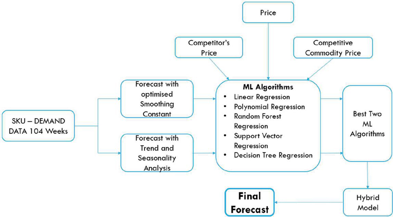
Figure 1 Flowchart of the adopted forecasting methodology.
Furthermore, by selecting a pair of regression algorithms from five algorithms, we have also created 10 more hybrid models (C). The results were compared for all five algorithms and hybrid models.
4 Results
The accuracy of various machine learning models depends upon several error estimate parameters such as the mean absolute deviation (MAD), mean squared error (MSE), Mean absolute percentage error (MAPE), Correlation coefficient, coefficient of determination, etc. For our model, we have considered MAPE, MAD, and MSE as the parameters for comparing models. The results are summarized in the table given below.
Table 1 Results for regression and hybrid algorithms
| MODEL | MAD | MSE | MAPE |
| Exponential Smoothing (Optimized Alpha) | 13.53 | 257.3 | 19.46 |
| LR | 5.95 | 59.26 | 8.45 |
| PR | 15.73 | 625.04 | 21.19 |
| RF | 5.69 | 53.97 | 8 |
| DTR | 8.03 | 127.26 | 11.11 |
| SVR | 11.7 | 194.82 | 17.01 |
| LR-PR | 5.74 | 55.22 | 8.26 |
| LR-RF | 5.42 | 47.87 | 7.76 |
| LR-DTR | 5.68 | 54.38 | 8.16 |
| LR-SVR | 5.52 | 51 | 7.95 |
| PR-DTR | 7.5 | 98.34 | 10.63 |
| PR-SVR | 7.52 | 99.13 | 10.71 |
| PR-RF | 5.9 | 56.41 | 8.39 |
| RF-SVR | 5.59 | 51.01 | 7.99 |
| DTR-SVR | 6.65 | 78.23 | 9.49 |
| RF-DTR | 5.87 | 59.7 | 8.33 |
| BEST and Second-Best Hybrid | 5.41 | 50.28 | 7.74 |
5 Discussion and Conclusion
Accurately forecasting demand is crucial for optimizing supply chain operations, particularly for retailers. In this study, we propose a hybrid model of machine learning algorithms to predict demand for each SKU of a retail store. To achieve this, we identified and assimilated the best two regression algorithms from a set of five regression algorithms. The hybrid model for the retail store is trained to enhance prediction accuracy compared to a single regression algorithm.
Table 1 reveals that among the five machine learning algorithms, the Random Forest regressor outperformed the rest with MAPE, MAD, and MSE values of 8%, 5.69, and 53.97, respectively, followed by Linear Regression with values of 8.45%, 5.95, and 59.26, respectively. Furthermore, when the same values were obtained for the traditional forecasting method, i.e., exponential smoothing (optimised smoothing constant), we concluded that machine learning algorithms are generally better than traditional methods for forecasting, although this is not always the case, as seen with Polynomial Regression.
When we compared the hybrid models with the individual regression algorithms that constitute the hybrid model, we found that in almost all cases (except for the PR-RF hybrid), the former performed better than the latter. Although there is not much significant difference between the PR-RF hybrid model and the RF algorithm, the PR-RF hybrid still outperformed the other four algorithms. The reason for the outperformance of hybrid models is that they can address the shortcomings of individual models.
Additionally, the results of the hybrid model from the best and second-best machine learning algorithms for each SKU show improved performance over the 10 different hybrid combinations, except for MSE for the LR-RF hybrid. Hence, we recommend training the data with the identified best and second-best algorithm for each SKU as a better approach for demand prediction.
The proposed hybrid model of machine learning algorithms can significantly improve demand forecasting accuracy for retailers. Managers can use our approach for reliable operations at low inventory costs. Moreover, the approach will allow them to optimize their purchase decision, inventory levels, production schedules, and resource allocation to meet customer demands.
However, the limitation of present study is that we have considered only few parameters such as price, competitor’s price and competitive commodity’s price whereas demand may be dependent on other parameters such as holidays, weekends, weather etc. This study may thus be extended by incorporating more parameters and exploring more advanced regression algorithms.
References
[1] Luis Aburto, Richard Weber, Improved supply chain management based on hybrid demand forecasts, Applied Soft Computing, Volume 7, Issue 1, 2007, Pages 136–144, ISSN 1568-4946, https://doi.org/10.1016/j.asoc.2005.06.001. (https://www.sciencedirect.com/science/article/pii/S1568494605000311).
[2] Sushil Punia, Konstantinos Nikolopoulos, Surya Prakash Singh, Jitendra K. Madaan and Konstantia Litsiou (2020) Deep learning with long short-term memory networks and random forests for demand forecasting in multi-channel retail, International Journal of Production Research, 58:16, 4964–4979, DOI: 10.1080/00207543.2020.1735666. (https://www.tandfonline.com/doi/full/10.1080/00207543.2020.1735666).
[3] Massimo Pacella, Gabriele Papadia, Evaluation of deep learning with long short-term memory networks for time series forecasting in supply chain management, Procedia CIRP, Volume 99, 2021, Pages 604–609, ISSN 2212-8271, https://doi.org/10.1016/j.procir.2021.03.081. (https://www.sciencedirect.com/science/article/pii/S2212827121003711).
[4] Nau R., Forecasting with moving averages (2014) Forecasting with Moving Averages, pp. 1–3, Cited 21 times. https://www.scopus.com/inward/record.uri?eid=2-s2.0-85043601148\&partnerID=40\&md5=c240c46f7140525d662649472cc1efdf. (https://www.scopus.com/record/display.uri?eid=2-s2.0-85043601148\&origin=inward\&txGid=40f299263bbaa50af2e32b1bb25dfb9e).
[5] Liljana Ferbar Tratar, Blaž Mojškerc, Aleš Toman, Demand forecasting with four-parameter exponential smoothing, International Journal of Production Economics, Volume 181, Part A, 2016, Pages 162–173, ISSN 0925-5273, https://doi.org/10.1016/j.ijpe.2016.08.004. (https://www.sciencedirect.com/science/article/pii/S0925527316301839).
[6] Mulhern, F. J., Williams, J. D., and Leone, R. P. (1998). Variability of brand price elasticities across retail stores: Ethnic, income, and brand determinants. Journal of Retailing, 74(3), 427–446. doi: 10.1016/s0022-4359(99)80103-1. (https://sci-hub.se/10.1016/s0022-4359(99)80103-1).
[7] Kimitoshi Sato, Katsushige Sawaki, A continuous-time dynamic pricing model knowing the competitor’s pricing strategy, European Journal of Operational Research, Volume 229, Issue 1, 2013, Pages 223–229, ISSN 0377-2217, https://doi.org/10.1016/j.ejor.2013.02.022. (https://www.sciencedirect.com/science/article/pii/S0377221713001550).
[8] Sethuraman, R., Srinivasan, V., and Kim, D. (1999). Asymmetric and Neighborhood Cross-Price Effects: Some Empirical Generalizations. Marketing Science, 18(1), 23–41. http://www.jstor.org/stable/193249. (Asymmetric and Neighborhood Cross-Price Effects: Some Empirical Generalizations on JSTOR).
[9] Kris Johnson Ferreira, Bin Hong Alex Lee, David Simchi-Levi (2015) Analytics for an Online Retailer: Demand Forecasting and Price Optimization. Manufacturing & Service Operations Management 18(1): 69–88. (https://doi.org/10.1287/msom.2015.0561).
[10] Yue, Liu et al. ‘Product Life Cycle Based Demand Forecasting by Using Artificial Bee Colony Algorithm Optimized Two-stage Polynomial Fitting’. 1 Jan. 2016 : 825–836. (https://ip.ios.semcs.net/articles/journal-of-intelligent-and-fuzzy-systems/ifs169014).
[11] Jakob Huber, Heiner Stuckenschmidt, Daily retail demand forecasting using machine learning with emphasis on calendric special days, International Journal of Forecasting, Volume 36, Issue 4, 2020, Pages 1420–1438, ISSN 0169-2070, https://doi.org/10.1016/j.ijforecast.2020.02.005. (https://www.sciencedirect.com/science/article/pii/S0169207020300224).
[12] Silaparasetti, Teja, Das Adhikari, Nimai, Domakonda, Nishanth, Garg, Rajat and Gupta, Gaurav. (2017). An Intelligent Approach to Demand Forecasting. (https://www.researchgate.net/publication/327225380\_An\_Intelligent\_Approach\_to\_Demand\_Forecasting).
[13] Yunishafira, A. (2018). Determining the Appropriate Demand Forecasting Using Time Series Method: Study Case at Garment Industry in Indonesia. KnE Social Sciences, 3(10), 553–564. https://doi.org/10.18502/kss.v3i10.3156. (https://knepublishing.com/index.php/Kne-Social/article/view/3156).
[14] Ravinder, Handanhal. (2016). Determining The Optimal Values Of Exponential Smoothing Constants – Does Solver Really Work?. American Journal of Business Education (AJBE). 9. 39. DOI: 10.19030/ajbe.v9i1.9574. (https://files.eric.ed.gov/fulltext/EJ1054363.pdf).
[15] Elcio Tarallo, Getúlio K. Akabane, Camilo I. Shimabukuro, Jose Mello, Douglas Amancio, Machine Learning in Predicting Demand for Fast-Moving Consumer Goods: An Exploratory Research, IFAC-PapersOnLine, Volume 52, Issue 13, 2019, Pages 737–742, ISSN 2405–8963, https://doi.org/10.1016/j.ifacol.2019.11.203. (https://www.sciencedirect.com/science/article/pii/S240589631931153X).
[16] Real Carbonneau, Kevin Laframboise, Rustam Vahidov, Application of machine learning techniques for supply chain demand forecasting, European Journal of Operational Research, Volume 184, Issue 3, 2008, Pages 1140–1154, ISSN 0377-2217, https://doi.org/10.1016/j.ejor.2006.12.004. (https://www.sciencedirect.com/science/article/pii/S0377221706012057).
[17] Punit Gupta et al. 2021 J. Phys.: Conf. Ser. 1714 012003. DOI: 10.1088/1742-6596/1714/1/012003. (https://iopscience.iop.org/article/10.1088/1742-6596/1714/1/012003).
[18] Luciano Viverit, Cindy Yoonjoung Heo, Luís Nobre Pereira, Guido Tiana, Application of machine learning to cluster hotel booking curves for hotel demand forecasting, International Journal of Hospitality Management, Volume 111, 2023, 103455, ISSN 0278-4319, https://doi.org/10.1016/j.ijhm.2023.103455. (https://www.sciencedirect.com/science/article/pii/S0278431923000294).
[19] Smirnov, P and Sudakov, Vladimir. (2021). Forecasting new product demand using machine learning. Journal of Physics: Conference Series. 1925. 012033. DOI: 10.1088/1742-6596/1925/1/012033. (https://www.researchgate.net/publication/352614910\_Forecasting\_new\_product\_demand\_using\_machine\_learning).
[20] Kologlu, Yunus, Birinci, Hasan, Ilgaz, Sevde and Ozyilmaz, Burhan. (2018). A Multiple Linear Regression Approach For Estimating the Market Value of Football Players in Forward Position. (https://arxiv.org/ftp/arxiv/papers/1807/1807.01104.pdf).
[21] Vaardini, Sindhu. (2015). An Assessment on the Building Demand Forecasting by Linear Regression Analysis. DOI: 10.13140/RG.2.1.1510.4484. (https://www.researchgate.net/publication/282003676\_An\_Assessment\_on\_the\_Building\_Demand\_Forecasting\_by\_Linear\_Regression\_Analysis).
[22] Martha Flores-Sosa, Ernesto León-Castro, José M. Merigó, Ronald R. Yager, Forecasting the exchange rate with multiple linear regression and heavy ordered weighted average operators, Knowledge-Based Systems, Volume 248, 2022, 108863, ISSN 0950-7051, https://doi.org/10.1016/j.knosys.2022.108863. (https://www.sciencedirect.com/science/article/pii/S0950705122004129).
[23] Noa Ohana-Levi, Alon Ben-Gal, Sarel Munitz, Yishai Netzer, Grapevine crop evapotranspiration and crop coefficient forecasting using linear and non-linear multiple regression models, Agricultural Water Management, Volume 262, 2022, 107317, ISSN 0378-3774, https://doi.org/10.1016/j.agwat.2021.107317. (https://www.sciencedirect.com/science/article/pii/S0378377421005941).
[24] Filippo Maria Ottaviani, Alberto De Marco, Multiple Linear Regression Model for Improved Project Cost Forecasting, Procedia Computer Science, Volume 196, 2022, Pages 808–815, ISSN 1877-0509, https://doi.org/10.1016/j.procs.2021.12.079. (https://www.sciencedirect.com/science/article/pii/S1877050921023024).
[25] Mutaz AlShafeey, Csaba Csáki, Evaluating neural network and linear regression photovoltaic power forecasting models based on different input methods, Energy Reports, Volume 7, 2021, Pages 7601–7614, ISSN 2352-4847, https://doi.org/10.1016/j.egyr.2021.10.125. (https://www.sciencedirect.com/science/article/pii/S2352484721011446)
[26] G. Ciulla, A. D’Amico, Building energy performance forecasting: A multiple linear regression approach, Applied Energy, Volume 253, 2019, 113500, ISSN 0306-2619, https://doi.org/10.1016/j.apenergy.2019.113500. (https://www.sciencedirect.com/science/article/pii/S0306261919311742).
[27] Aliyeh Kazemi, Amir Foroughi. A, Mahnaz Hosseinzadeh, A Multi-Level Fuzzy Linear Regression Model for Forecasting Industry Energy Demand of Iran, Procedia – Social and Behavioral Sciences, Volume 41, 2012, Pages 342–348, ISSN 1877-0428, https://doi.org/10.1016/j.sbspro.2012.04.039. (https://www.sciencedirect.com/science/article/pii/S1877042812009196).
[28] Metin İfraz, Adnan Aktepe, Süleyman Ersöz, Tahsin Çetinyokuş, Demand forecasting of spare parts with regression and machine learning methods: Application in a bus fleet, Journal of Engineering Research, Volume 11, Issue 2, 2023, 100057, ISSN 2307-1877, https://doi.org/10.1016/j.jer.2023.100057. (https://www.sciencedirect.com/science/article/pii/S2307187723000585).
[29] S. Thomas Ng, Martin Skitmore, Keung Fai Wong, Using genetic algorithms and linear regression analysis for private housing demand forecast, Building and Environment, Volume 43, Issue 6, 2008, Pages 1171–1184, ISSN 0360-1323, https://doi.org/10.1016/j.buildenv.2007.02.017. (https://www.sciencedirect.com/science/article/pii/S0360132307000923).
[30] Sushil Punia, Sonali Shankar, Predictive analytics for demand forecasting: A deep learning-based decision support system, Knowledge-Based Systems, Volume 258, 2022, 109956, ISSN 0950-7051, https://doi.org/10.1016/j.knosys.2022.109956. (https://www.sciencedirect.com/science/article/pii/S0950705122010498).
[31] Sunthornjittanon, Supichaya, “Linear Regression Analysis on Net Income of an Agrochemical Company in Thailand” (2015). University Honors Theses. Paper 131. https://doi.org/10.15760/honors.137. https://pdxscholar.library.pdx.edu/cgi/viewcontent.cgi?article=1156\&context=honorstheses.
[32] Ostertagova, Eva. (2012). Modelling Using Polynomial Regression. Procedia Engineering. 48. 500–506. DOI: 10.1016/j.proeng.2012.09.545. https://www.researchgate.net/publication/256089416\_Modelling\_Using\_Polynomial\_Regression/citation/download.
[33] Chu, F.-L. (2004). Forecasting tourism demand: a cubic polynomial approach. Tourism Management, 25(2), 209–218. doi: 10.1016/s0261-5177(03)00086-4. https://sci-hub.se/10.1016/S0261-5177(03)00086-4.
[34] Mahdi Abolghasemi, Eric Beh, Garth Tarr, Richard Gerlach, Demand forecasting in supply chain: The impact of demand volatility in the presence of promotion, Computers & Industrial Engineering, Volume 142, 2020, 106380, ISSN 0360-8352, https://doi.org/10.1016/j.cie.2020.106380. (https://www.sciencedirect.com/science/article/pii/S0360835220301145).
[35] Galina Merkuryeva, Aija Valberga, Alexander Smirnov, Demand forecasting in pharmaceutical supply chains: A case study, Procedia Computer Science, Volume 149, 2019, Pages 3–10, ISSN 1877-0509, https://doi.org/10.1016/j.procs.2019.01.100. (https://www.sciencedirect.com/science/article/pii/S1877050919301061).
[36] Jing Shi, Application of the model combining demand forecasting and inventory decision in feature-based newsvendor problem, Computers & Industrial Engineering, Volume 173, 2022, 108709, ISSN 0360-8352, https://doi.org/10.1016/j.cie.2022.108709. (https://www.sciencedirect.com/science/article/pii/S0360835222006970).
[37] David L. Banks, Stephen E. Fienberg- Polynomial Regression in Encyclopedia of Physical Science and Technology (Third Edition), 2003. https://www.sciencedirect.com/topics/computer-science/polynomial-regression.
[38] Loh, Wei-Yin. (2011). Classification and Regression Trees. Wiley Interdisciplinary Reviews: Data Mining and Knowledge Discovery. 1. 14–23. DOI: 10.1002/widm.8. https://www.researchgate.net/publication/227658748\_Classification\_and\_Regression\_Trees.
[39] Kris Johnson Ferreira, Bin Hong Alex Lee, David Simchi-Levi Analytics for an Online Retailer: Demand Forecasting and Price Optimization. https://www.hbs.edu/ris/Publication\%20Files/kris\%20Analytics\%20for\%20an\%20Online\%20Retailer\_6ef5f3e6-48e7-4923-a2d4-607d3a3d943c.pdf.
[40] Ida Rezaei, Seyed Hossein Amirshahi, Ali Akbar Mahbadi, Utilizing support vector and kernel ridge regression methods in spectral reconstruction, Results in Optics, Volume 11, 2023, 100405, ISSN 2666-9501, https://doi.org/10.1016/j.rio.2023.100405. (https://www.sciencedirect.com/science/article/pii/S2666950123000573).
[41] Congjun Rao, Yue Zhang, Jianghui Wen, Xinping Xiao, Mark Goh, Energy demand forecasting in China: A support vector regression-compositional data second exponential smoothing model, Energy, Volume 263, Part C, 2023, 125955, ISSN 0360-5442, https://doi.org/10.1016/j.energy.2022.125955. (https://www.sciencedirect.com/science/article/pii/S0360544222028419).
[42] Chi-Jie Lu, Yen-Wen Wang, Combining independent component analysis and growing hierarchical self-organizing maps with support vector regression in product demand forecasting, International Journal of Production Economics, Volume 128, Issue 2, 2010, Pages 603–613, ISSN 0925-5273, https://doi.org/10.1016/j.ijpe.2010.07.004. (https://www.sciencedirect.com/science/article/pii/S092552731000229X).
[43] A.A. Levis, L.G. Papageorgiou, Customer Demand Forecasting via Support Vector Regression Analysis, Chemical Engineering Research and Design, Volume 83, Issue 8, 2005, Pages 1009–1018, ISSN 0263-8762, https://doi.org/10.1205/cherd.04246. (https://www.sciencedirect.com/science/article/pii/S0263876205727945).
[44] Wang Guanghui, Demand Forecasting of Supply Chain Based on Support Vector Regression Method, Procedia Engineering, Volume 29, 2012, Pages 280–284, ISSN 1877-7058, https://doi.org/10.1016/j.proeng.2011.12.707. (https://www.sciencedirect.com/science/article/pii/S1877705811065441)
[45] Robin Singh Bhadoria, Manish Kumar Pandey, Pradeep Kundu, RVFR: Random vector forest regression model for integrated & enhanced approach in forest fires predictions, Ecological Informatics, Volume 66, 2021, 101471, ISSN 1574-9541, https://doi.org/10.1016/j.ecoinf.2021.101471. (https://www.sciencedirect.com/science/article/pii/S1574954121002624).
[46] Sehoon Kim, Innovating knowledge and information for a firm-level automobile demand forecast system: A machine learning perspective, Journal of Innovation & Knowledge, Volume 8, Issue 2, 2023, 100355, ISSN 2444-569X, https://doi.org/10.1016/j.jik.2023.100355. (https://www.sciencedirect.com/science/article/pii/S2444569X23000513).
[47] R.M. van Steenbergen, M.R.K. Mes, Forecasting demand profiles of new products, Decision Support Systems, Volume 139, 2020, 113401, ISSN 0167-9236, https://doi.org/10.1016/j.dss.2020.113401. (https://www.sciencedirect.com/science/article/pii/S0167923620301561).
[48] Matthias Ulrich, Hermann Jahnke, Roland Langrock, Robert Pesch, Robin Senge, Distributional regression for demand forecasting in e-grocery, European Journal of Operational Research, Volume 294, Issue 3, 2021, Pages 831–842, ISSN 0377-2217, https://doi.org/10.1016/j.ejor.2019.11.029. (https://www.sciencedirect.com/science/article/pii/S0377221719309403).
[49] Takashi Tanizaki, Tomohiro Hoshino, Takeshi Shimmura, Takeshi Takenaka, Restaurants store management based on demand forecasting, Procedia CIRP, Volume 88, 2020, Pages 580–583, ISSN 2212-8271, https://doi.org/10.1016/j.procir.2020.05.101. (https://www.sciencedirect.com/science/article/pii/S2212827120304236).
[50] Abigail Bola Adetunji, Oluwatobi Noah Akande, Funmilola Alaba Ajala, Ololade Oyewo, Yetunde Faith Akande, Gbenle Oluwadara, House Price Prediction using Random Forest Machine Learning Technique, Procedia Computer Science, Volume 199, 2022, Pages 806–813, ISSN 1877-0509, https://doi.org/10.1016/j.procs.2022.01.100. (https://www.sciencedirect.com/science/article/pii/S1877050922001016).
[51] D. Rohaan, E. Topan, C.G.M. Groothuis-Oudshoorn, Using supervised machine learning for B2B sales forecasting: A case study of spare parts sales forecasting at an after-sales service provider, Expert Systems with Applications, Volume 188, 2022, 115925, ISSN 0957-4174, https://doi.org/10.1016/j.eswa.2021.115925. (https://www.sciencedirect.com/science/article/pii/S0957417421012793).
[52] Juan D. Díaz, Erwin Hansen, Gabriel Cabrera, A random walk through the trees: Forecasting copper prices using decision learning methods, Resources Policy, Volume 69, 2020, 101859, ISSN 0301-4207, https://doi.org/10.1016/j.resourpol.2020.101859. (https://www.sciencedirect.com/science/article/pii/S0301420720308904).
[53] Yifei He, Chao Chen, Bin Li, Zili Zhang, Prediction of near-surface air temperature in glacier regions using ERA5 data and the random forest regression method, Remote Sensing Applications: Society and Environment, Volume 28, 2022, 100824, ISSN 2352-9385, https://doi.org/10.1016/j.rsase.2022.100824. (https://www.sciencedirect.com/science/article/pii/S235293852200132X).
[54] Robin Singh Bhadoria, Manish Kumar Pandey, Pradeep Kundu, RVFR: Random vector forest regression model for integrated & enhanced approach in forest fires predictions, Ecological Informatics, Volume 66, 2021, 101471, ISSN 1574-9541, https://doi.org/10.1016/j.ecoinf.2021.101471. (https://www.sciencedirect.com/science/article/pii/S1574954121002624).
[55] Seungmi Kwak, Jaehwang Kim, Hongsheng Ding, Xuesong Xu, Ruirun Chen, Jingjie Guo, Hengzhi Fu, Machine learning prediction of the mechanical properties of -TiAl alloys produced using random forest regression model, Journal of Materials Research and Technology, Volume 18, 2022, Pages 520–530, ISSN 2238-7854, https://doi.org/10.1016/j.jmrt.2022.02.108. (https://www.sciencedirect.com/science/article/pii/S2238785422002800).
[56] Mitra, A., Jain, A., Kishore, A. et al. A Comparative Study of Demand Forecasting Models for a Multi-Channel Retail Company: A Novel Hybrid Machine Learning Approach. Oper. Res. Forum 3, 58 (2022). https://doi.org/10.1007/s43069-022-00166-4. https://link.springer.com/article/10.1007/s43069-022-00166-4.
Biographies

Vinit Taparia did his B.Tech in Mechanical Engineering from Malaviya National Institute of Technology, Jaipur, Rajasthan. Currently he is working on Gas and Power Projects. His research interests include supply chain management, demand planning, inventory management, and renewable energy sources.

Piyush Mishra completed his B.Tech in Mechanical Engineering from Malaviya National Institute of Technology Jaipur, Rajasthan. He is currently employed in Reliance Industries in FCC unit of DTA Refinery. His research interests include supply chain management, demand planning, inventory management and planning.

Nitik Gupta completed his B.Tech in Mechanical engineering from Malaviya National Institute of Technology, Jaipur, Rajasthan. He is currently employed in Fernweh Group, a private equity firm as an Analyst focusing on Industrials sector and its sub-sectors. His research interests include supply chain management, demand planning & inventory management.

Devesh Kumar did his B.Tech in Mechanical Engineering from IIITDM Jabalpur, M.Tech from MNIT Jaipur. He is currently pursuing Ph.D. in Mechanical Engineering from MNIT Jaipur. His research interests lie in the domains of supply chain management, machine learning, decision-making, and optimization techniques.
Journal of Graphic Era University, Vol. 12_1, 15–36.
doi: 10.13052/jgeu0975-1416.1212
© 2023 River Publishers